Following up on my previous post, attached is a fully vectorized version of my original prediction function, which is extremely efficient, and basically instantaneous. Also attached is a command line script that demonstrates how to use it.
Uncategorized
Vectorized Clustering Algorithm
Attached is a completely vectorized, highly efficient version of my original clustering algorithm. Its runtime is drastically shorter, and comparable to my real-time algorithms, though it is based upon my original technique of iterating through different levels of discernment until we find the level that generates the greatest change in the entropy of the categorization. Also attached is a command line script that demonstrates how to apply it to a dataset.
Tracking Moving Objects in 3-Space
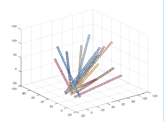
Attached is a polynomial-time algorithm that can identify, and then track objects in three-space over time given 3-D point information from a sensor, or other input.
Because the algorithm tracks at the point level, rather than at the object level (i.e., it builds its own objects from point data), it can be used to track objects that have irregular, and even diffuse shapes, like smoke, or steam.
Running on a $200 dollar laptop, it can track 15 Newtonian projectiles at a rate of about 3 frames per second, with an accuracy of about 98% to 100%.
Here’s a plot of one of the sets of projectiles I applied it to:
All of the other functions you need can be found in my full library here.
Autonomous Noise Filtering
I’ve updated Prometheus to include autonomous noise filtering.
This means that you can give it data that has dimensions that you’re not certain contribute to the classification, and might instead be noise. This allows Prometheus to take datasets that might currently produce very low accuracy classifications, and autonomously eliminate dimensions until it produces accurate classifications.
It can handle significant amounts of noise:
I’ve given it datasets where 50% of the dimensions were noise, and it was able to uncover the actual dataset within a few minutes.
In short, you can give it garbage, and it will turn into gold, on its own.
Since I’ve proven that it’s basically mathematically impossible to beat nearest neighbor using real-world Euclidean data, and I’ve come up with a vectorized implementation of nearest neighbor, this version of Prometheus uses only nearest neighbor-based methods.
As a result, the speed is insane.
If you don’t use filtering, classifications occur basically instantaneously on a cheap laptop. If you do have some noise, it still takes only a few minutes for a dataset of a few hundred vectors to be processed, even on a cheap laptop.
Attached should be all the code you need to run it, together with a command line script that demonstrates how to use it. But, it’s probably easier to simply download the my full library as a zip file from my researchgate blog.
Enjoy, and if you’re interested in a commercial version, please let me know.
On Nearest Neighbor
I’ve been using nearest neighbor quite a bit lately, and I’ve noticed that its accuracy is remarkable, and I’ve been trying to understand why.
It turns out that you can prove that for certain datasets, you actually can’t do better than the nearest neighbor algorithm:
Assume that for a given dataset, classifications are constant within a radius of R of any data point.
Also assume that each point has a neighbor that is within R.
That is, if x is a point in the dataset, then there is another point y in the dataset such that ||x-y|| < R.
In plain terms, classifications don’t change unless you travel further than R from a given data point, and every point in the dataset has a neighbor that is within R of that point.
Now let’s assume we’re given a new data point from the testing set that is within the boundaries of the training set.
By definition, the new point is within R of some point from the training set, which implies it has the same class as that point from the training set.
This proves the result.
This means that given a sufficiently dense, locally consistent dataset, it is mathematically impossible to make predictions that are more accurate than nearest neighbor, since it will be 100% accurate in this case.
Unless you’re doing discrete mathematics, which can be chaotic (e.g., nearest neighbor obviously won’t work for determining whether a number is prime) your dataset will probably be locally consistent for a small enough value of R.
And since we have the technology to make an enormous number of observations, we can probably produce datasets that satisfy the criteria above.
The inescapable conclusion is that if you have a sufficiently large number of observations, you can probably achieve a very high accuracy simply using nearest neighbor.
On Classifications
I’ve been doing some thinking about the mathematics and theory of classifications, as opposed to actually implementing particular classifications, and I’ve come to a few conclusions that I thought I’d share, in advance of a formal article.
The initial observation comes from the nearest neighbor technique that I’ve been making use of lately: given a dataset, and an input vector, the nearest neighbor algorithm uses the class of the vector that is most similar to the input vector as predictive of the class of the input vector. In short, if you want to predict what the class of a given input vector is, you use the class of the vector to which the input vector is most similar. This is generally measured using the Euclidean norm operator, but you could substitute other operators as well depending upon the context. This method works astonishingly well, and can be implemented very efficiently using vectorized languages like MATLAB and Octave.
The assumption that underlies this model is that the space in which the data exists is locally consistent. That is, there is some sufficiently small neighborhood around any given point, within which all points have the same classifier. The size of this neighborhood is arguably the central question answered by my initial paper on Artificial Intelligence, if we interpret the value of 
However, there are very simple examples where this assumption fails, such as the distinction between odd and even numbers. In fact, using the nearest neighbor approach will by definition produce an incorrect answer every time, since the nearest neighbor of an even number is an odd number, and the nearest neighbor of an odd number is an even number. Music is another example where the space is simply not locally consistent, and as a result, substituting a note with its nearest neighbor can produce disastrous results.
We can instead add additional criteria that would allow us to describe these spaces. For example, if we want to determine whether a given input integer is an even or an odd number, we can use an algorithm that searches for numbers within the dataset that have a distance from the input vector of exactly two. Similarly, we could require some minimum distance, and set a maximum distance. That is, vectors 


The question is whether we can infer the correct function given the dataset, which might not always be the case. That is, even if there is some computable function that allows us to say whether two points have the same classifier, we might not have enough data to determine whether or not this is the case. That is, the correct function might rely upon information that is exogenous to the dataset itself. Finally, this also suggests the question of whether it is decidable on a UTM (x) that we in fact have enough information to derive the correct function for the dataset in question, and if so, (y) whether or not there is a computable process that generates the correct function.
Minimalist Image Partition Algorithm
Attached is a very stripped down image partition algorithm, together with a command line script that demonstrates how to use it.
Discerning Objects in 3-Space
Below is an algorithm that can, in polynomial time, identify objects in a three-dimensional space given point information about the objects in the scene. In short, it takes a set of points in Euclidean 3-space, and clusters them into individual objects. The technique is essentially identical to that used by my original image partition algorithm, but rather than cluster regions in an image, this algorithm clusters points in 3-space.
The algorithm is intended to take in points from sensor data, and then assemble those points into objects that can then be tracked as a whole. The algorithm can be easily generalized to higher-dimensional spaces, but it’s meant to be a proper computer vision algorithm, so it’s written to work in 3-space. In a follow up article, I’ll present a similar algorithm that does the same over time, thereby tracking points over time as individual objects in 3-space. This can be done by taking each point in a given moment in time, and finding its nearest neighbor in the next moment in time.
Here’s the code, together with a command line script that runs a simple example:
Optimized Image Delimiter
Attached is another version of my image delimiter algorithm, that iterates through different grid sizes, selecting the grid size that generates the greatest change in the entropy of the resultant image partition.
It’s essentially a combination of my original image partition algorithm and my image delimiter algorithm. I’m still tweaking it, but it certainly works as is.
Using Light to Implement Deep Learning
The electromagnetic spectrum appears to be arbitrarily divisible. This means that for any subset of the spectrum, we can subdivide that subset into an arbitrarily large number of intervals. So, for example, we can, as a theoretical matter matter, subdivide the visible spectrum into as many intervals as we’d like. This means that if we have a light source that can emit a particular range of frequencies, and a dataset that we’d like to encode using frequencies of light from that range, we can assign each element of the dataset a unique frequency.
So let’s assume we have a dataset of 


If we shine two beams of light, each with their own frequency, through a refractive medium, like a prism, then the exiting angle of those beams will be different. As a result, given an input vector, and a dataset of vectors, all of which are then encoded as beams of light, it should be very easy to find which vector from the dataset is most similar to the input vector, using some version of refraction, or perhaps interferometry. This would allow for nearest-neighbor deep learning to be implemented using a computer driven by light, rather than electricity.
I’ve already shown that vectorized nearest-neigbor is an extremely fast, and accurate method of implementing machine learning. Perhaps by using a beam-splitter, we can simultaneously test an input vector against an entire dataset, which would allow for something analogous to vectorization using beams of light.
