Friday evening I went on a tirade on Twitter about an idea I had for a robot a while back, but the core point has nothing to do with robotics itself, and is really about imitation. Specifically, what I said was, let’s imagine you have a machine that has a set of physical controls capable of executing incremental physical change. For example, the signal causes a piston to lift some marginal distance. There is therefore in every case a set of signals , and their resultant motions. Let’s assume the machine in question can compare its own current state to the state of some external system it’s trying to imitate, which could of course be a dataset. Returning to the previous example, imagine a machine trying to imitate a pumping motion –
It would then compare the motions of the piston to the motions in the dataset that describe that desired motion in question, and this will produce some measure of distance.
Now imagine a control system that fires the appropriates motions in order when given the vector . If there are possible signals, and therefore possible motions, then we can use a Monte Carlo simulator to generate a large number of vectors, in parallel, and therefore, a large number of motions. The machine can then test the incremental change that occurs as a result of executing the sequence encoded in each resultant , and compare it to the motions it’s trying to imitate, again in parallel. Obviously, you select the motion that minimizes the difference between the desired motion and the actual motion, and if you need tie-breakers, you look to the standard deviation of velocities, or the entropies of the velocities, each of which should help achieve smoothness. This obviously requires the machine to have a model of its own state, but you could also imagine a factory floor filled with the same machines, all learning from each other –
This happens anyway, so why not utilize the fact that you have a bunch of the same machines in the same place, to allow them to actually test motions, physically, in parallel. This would be the case where outcome is measured, rather than modeled. This could prove quite powerful, because you don’t need a machine to calculate what’s going to happen, but instead, the machine can rely upon observation, piggybacking off of the computational power of Nature itself. If what’s going to happen is complex, and therefore computationally intensive, this could prove extremely useful, because you can achieve true parallelization through manufacturing that’s going to happen anyway, if you’re producing at scale. I had this idea a while back, regarding engines, but the more general idea seems potentially quite powerful.
We can apply the same kind of optimizer I used in classifications in this process, which should allow us to navigate the state space of motions efficiently.
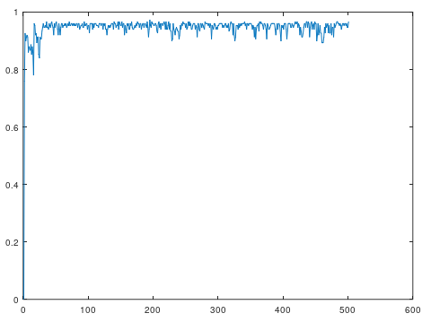
Following up on my note from yesterday, I’ve tweaked the interpolation algorithm, now making use of a simple optimizer that takes the best answer for a given iteration, and narrows the range of the Monte Carlo simulations around it based upon the accuracy, iteratively winnowing down the range and zooming in on a best solution. It works really well, and it’s really fast, achieving 97.3% accuracy in .34 seconds on the UCI Iris dataset. You can tweak the parameters, going for deeper simulations, more simulations per iteration, etc, but this already plainly works. I’ll follow up with one more article on this method as applied to the MNIST Fashion Dataset, since that’s what prompted my curiosity on the matter, at least recently.
Here’s a plot of the accuracy as a function of simulation depth (i.e., the number of times the underlying Monte Carlo simulator is called). This version of the optimizer simply allocates all of the parallel capacity to the best answer, and adjusts the width of the range in which it searches based upon accuracy. However, you could of course also imagine a version where you allocate capacity in proportion to accuracy. That is, rather than compute around only the best answer, compute around all answers, with the amount of computation around an answer determined by the accuracy of the answer.
I’ve been playing with these algorithms, and it turns out they’re terrible on certain datasets, which led me to ask why, and the answer is rather obvious:
Because the underlying interpolation is linear, assume that you have two points in the dataset and , for which the correct classifications are the same. If the coefficient for the y-dimension is non-zero, then we can fix , and increase arbitrarily, and at some point, we’re going to change the resultant classifier of the function .
I think the takeaway is, this could be useful for some datasets that are not locally consistent, but that doesn’t mean it’s useful for the complement of the set of locally consistent datasets, but is instead useful for some of them.
It just dawned on me that by mapping to a single classifier, you are destroying information. It instead could be better to map from one Euclidean space to another of the same or higher dimension.
For example, a linear function could map a vector in N-dimensions to another of N-dimensions, with the goal to map vectors of the same class to roughly the same region of the new second space. This of course assumes the original dataset is not locally consistent, otherwise you could just use distance-based clustering.
Moreover, you could map pairs of feature values using a second degree polynomial, and so on, which would take an input vector and map it to a higher dimensional space, again, with the goal of maximizing the classification consistency of that second Euclidean space.
For example, here’s an algorithm that I’m going to code over the next couple days:**
1. Count the number of classes in the dataset, assign each a label from 1 to K.
2. Randomly generate origins for each of the K classes of data in N-space, where N is the dimension of the dataset, such that none of the spheres of radius 1 from each such origin overlap (i.e., generate K non-intersecting spheres of radius 1 in N-space).*
3. Assign each class of vectors a unique origin / sphere.
4. Test for the Euclidean distance between each point in a given class and its assigned origin, and take the total distance for each point, over all classes; do this for each randomly generated set of origins.
5. Select the set of origins that minimizes the total distance calculated in Step 4.
6. Now given the set of origins that minimizes the distance calculated in Step 4, use a Monte Carlo simulation / optimizer to generate an equation (e.g., linear, polynomial, etc.) that maps each point in a given class to a point in its associated sphere.
The net effect of this algorithm is to map possibly locally inconsistent data to a locally consistent space (i.e., a set of non-overlapping spheres that contain only one class of data).
*In some cases you might be able to use fewer dimensions, and in others, you might have to use more, because for example you’re making use of combinations of feature values, which would require additional dimensions in the output space. We could also take a “center of mass approach” for each class, which would save time, and simply assign each class an origin equal to the average value over the vectors in the class, and then size the radius so there’s no overlap.
** The more general idea here seems quite promising, which is that it’s a set of operations that bring you from an initial state to some desired goal state, that is perhaps quite different from the initial state, and is solved for using parallel operations. It is in essence, in this view, a vectorized state space algorithm.
Following up on my note from a few days ago, below is Matlab / Octave code that implements interpolated classifications. I’ve tested it on only the UCI Iris dataset, but it works, and because it’s not deterministic, the accuracy varies, and seems to range from 82% to 92%, given 350,000 Monte Carlo simulations. It’s slower than my core algorithms, but it’s still fast, and runs in 2 to 10 seconds, but starts to slow down as you increase the number of simulations.
Again, this is useful, because this algorithm does not require the data to be locally consistent (i.e., classifications can vary over small distances). This allows for classifications of datasets that might have e.g., arbitrary classifiers made up by a human, rather than a truly intrinsic classification structure.
In a previous article, I introduced a vectorized method for achieving interpolation, which works quite well, and is very fast. I abandoned it because I had other things getting my attention, including, maximizing the use of vectorization in my core algorithms, because it really changes their runtimes. I’ve also proven that you can’t beat the accuracy of my algorithms for a class of datasets that I’ve rigorously defined as, “locally consistent” datasets. The gist is, if classifications don’t change much over small distances, then the dataset is locally consistent. Because my core algorithms are also have linear runtimes, that’s pretty much the end of the story for locally consistent datasets, which probably covers a significant chunk of real world datasets.
So, I’ve started to think about datasets that are not locally consistent, and what’s interesting, is that the MNIST Fashion dataset seems to have some inconsistent classes, because my algorithms have really high accuracy overall for MNIST Fashion, but have randomly horrible accuracy for certain rows (but not enough to push the overall accuracy down too much). So I’m now turning my attention to using interpolation, i.e., constructing a function that takes the features in a dataset, and calculates its class.
Before I decided to do this, I wanted to make sure that I wasn’t wasting my time, and creating something that is only superficially different from what I’ve already done, but mathematically equivalent. And it turns out, it is not the same as the distance-based clustering and prediction I’ve made use of so far. Specifically, it doesn’t require the same features to have similar values, which my current algorithms do –
It instead requires that the function returns the same value when evaluated for two elements of the same class. As a result, I’m going to spend a few days on this, because it is new, and perhaps it’s useful, and could provide a more efficient method of implementing what is a basically neural network.
I noted on Twitter that I came up with a really efficient way of calculating spatial entropy, and though I plan on writing something more formal on the topic, as it’s related to information theory generally, I wanted to at least write a brief note on the method, which is as follows:
Let be a set of points in Euclidean -space. Sort them by row value, which will produce a sorted matrix of vectors . Now take the norm of the difference between all adjacent entries, , which will produce a vector of real numbers, that correspond to the norms of those differences. Let be the sum over the entries in the vector , and take the entropy of the vector , which will correspond to a distribution.
So for example, if you have points along a line, and all of them are equidistant from one another, then the entropy will be equal to the , which corresponds to a uniform distribution, which is consistent with intuition, since you’d expect entropy to be maximized. In contrast, if all points are at the same location, then their distances would be zero, and the entropy would be zero.
You could do the same with a set of curves, but you’d need a comparison operator to first sort the curves and then compare their distances, and for this, you can use the operators I used in Section 1.3 of my A.I. summary (the “Expanding Gas Dataset”).
This allows for the measurement of the the entropy of an arbitrary dataset of vectors.
Information, Knowledge, and Uncertainty
The fundamental observation I’ve made regarding uncertainty, is that what you know about a system plus what you don’t, is all there is to know about the system. This sounds tautological, but so is the founding equation of accounting, which was also founded by an Italian mathematician, which it seems clear people are trying to forget.
Expressed symbolically, the equation states that:
,
Where is the information content of the system, is your knowledge with respect to the system, and is your uncertainty with respect to the system. I go through some examples in this note on the matter, but the intuition should be straightforward.
Because we can now measure spatial entropy, we can measure the entropy of a dataset, which would also be the information content, , of the dataset, but let’s table that for a moment.
My prediction algorithms return a set of vectors given an input vector, and it allows for blank entries in the input vector. So if you observe the first 50 out of 1,000 states of a system, you’ll get a set of vectors that reflect the information you have, and of course, that set winnows down in size as the number of observations increases (see Section 3.1 of A New Model of Artificial Intelligence).
Here’s a representative chart (from that paper) that shows how the set of possible paths of a random walk starts to tilt in favor of an upward path as data becomes available. In this case, 2,000 observations are available out of 10,000, and the input vector is in fact an upward tilting path.
We can also measure the entropy of this set of returned set of predictions, using the same method described above, which would in my opinion represent your uncertainty with respect to your prediction. This makes sense, because in the worst case, you get back the full training dataset, which would set your uncertainty equal to the information content of the dataset. Expressed symbolically,
.
This implies that your knowledge with respect to your prediction is zero, which is correct. That is, if your prediction algorithm says, my prediction is, the entire training dataset, then it doesn’t know anything at all. As observations become available, the set of returned predictions will shrink in size, which will reduce the entropy of the returned prediction set, implying non-zero knowledge. Eventually, you could be left with a single prediction, which would imply perfect knowledge, and no uncertainty, in the context of your training dataset, which is all you ever know about a given problem.


 and
and  , for which the correct classifications are the same. If the coefficient for the y-dimension is non-zero, then we can fix
  arbitrarily, and at some point, we’re going to change the resultant classifier of the function
  .
. be a set of
  -space. Sort them by row value, which will produce a sorted
  matrix of vectors
  . Now take the norm of the difference between all adjacent entries,
  , which will produce a
  vector
  of real numbers, that correspond to the norms of those differences. Let
  be the sum over the entries in the vector
  , which will correspond to a distribution.
 , which corresponds to a uniform distribution, which is consistent with intuition, since you’d expect entropy to be maximized. In contrast, if all points are at the same location, then their distances would be zero, and the entropy would be zero.
 ,
, is the information content of the system,
  is your uncertainty with respect to the system. I go through some examples
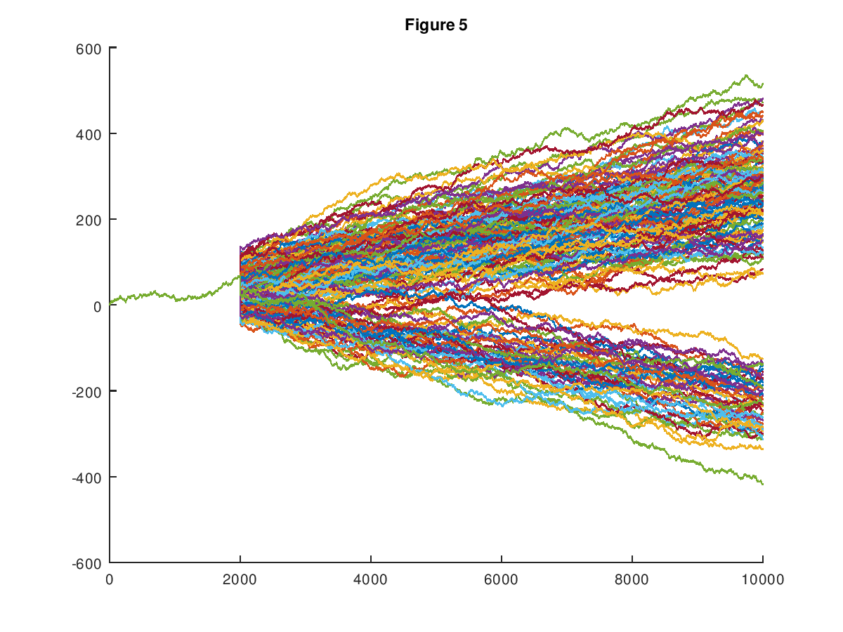
 .
.