I will continue to post academic updates to ResearchGate, and this blog, though the website will contain the actual releases of new software going forward.
I’m pleased to announce that after years of basically non-stop research and coding, I’ve completed the Free Version of my AutoML software, Black Tree (Beta 1.0). The results are astonishing, producing consistently high accuracy, with simply unprecedented runtimes, all in an easy to use GUI written in Swift for MacOS (version 10.10 or later):
Dataset
Accuracy
Total Runtime (Seconds)
UCI Credit (2,500 rows)
98.46%
217.23
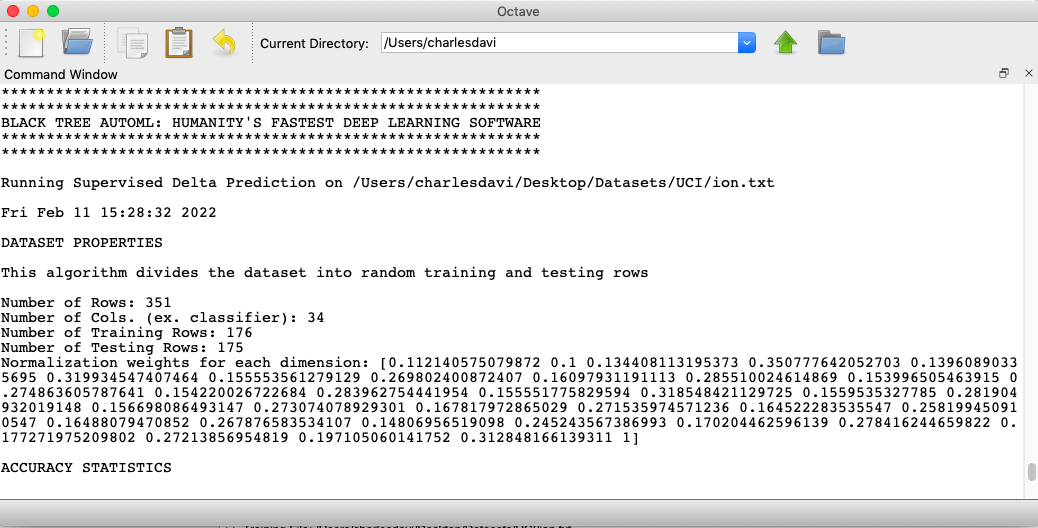
UCI Ionosphere (351 rows)
100.0%
0.7551
UCI Iris (150 rows)
100.0%
0.2379
UCI Parksinsons (195 rows)
100.0%
0.3798
UCI Sonar (208)
100.0%
0.5131
UCI Wine (178)
100.0%
0.3100
UCI Abalone (2,500 rows)
100.0%
10.597
MNIST Fashion (2,500 images)
97.76%
25.562
MRI Dataset (1,879 images)
98.425%
36.754
The results above were generated using Black Tree (Beta 1.0), applying the “Supervised Delta Prediction” algorithm to each of the datasets listed above, and you can download these datasets in a ready-to-use format from DropBox (UCI Datasets, MNIST Fashion, MRI Dataset).
The Free Version (Beta 1.0) is of course limited, but nonetheless generous, allowing for non-commercial classification and clustering, including image classification, for any dataset with no more than 2,500 rows / images. The Pro Version will include nearly my entire A.I. library, for just $199 per user per year, with no limit on the number of rows, allowing you to classify and cluster datasets with tens of millions of rows, in polynomial time, on a consumer device, without cloud computing or a data scientist (see Vectorized Deep Learning, generally). You can also purchase a lifetime commercial license of the Pro Version for just $1,000 per user.
INSTALLATION
You can download the executable file from the Black Tree website (11.1 MB). This can be placed anywhere you like on your machine, though upon opening the application, it will automatically create directories in “/Users/[yourname]/Documents/BlackTree”. Because of MacOS security settings, the first time you run Black Tree, you will have to right-click the application icon, and select “Open”, which should cause a notice to pop up (eventually), saying you downloaded the application from the Internet, and you want to open it anyway.
You must also download and install Octave, which is free, and available here, which will also require you to right-click the application file for security reasons (for the first time only). Then, you must install Octave’s image package (if you want to run image classification), which can be done by typing the following code into Octave’s command line:
pkg install -forge image
If for whatever reason, the package fails to download (e.g., no internet connection), then you can manually install the image package by downloading it from SourceForge, and then typing the following code into Octave’s command line:
pkg install [local_filename],
where “local_filename” is the full path and filename to the image package on your machine.
When you open Black Tree for the first time, it will automatically generate all of the necessary Octave command line code for you (including the code above), and copy it to your clipboard, so all you have to do is open Octave, and press CTRL + V to complete installation of Black Tree. Note that Black Tree will also automatically download Octave source code and sample datasets the first time you run it, so there will be some modest delay (only the first time) before you see the Black Tree GUI pop up.
RUNNING BLACK TREE
Data Classification / Clustering
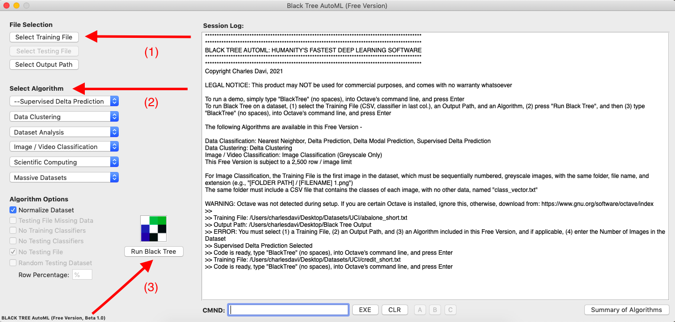
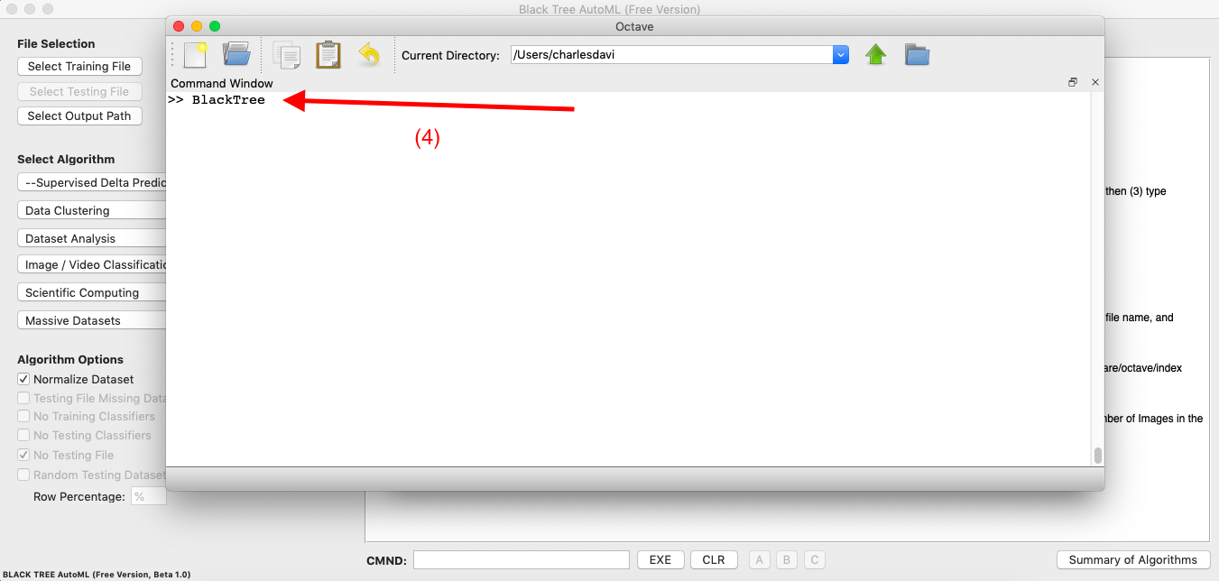
To run Data Classification / Clustering, simply (1) select a Training File and Output Path, (2) select an Algorithm, (3) press “Run Black Tree”, then (4) type “BlackTree”, no spaces, into Octave’s command line, and press Enter, that’s it. Note that the Free Version does not allow you to select both a training and testing file, and instead runs the selected algorithm on a single dataset. The exception is Supervised Delta Prediction, which automatically spilts the selected dataset exactly in half, into random training and testing datasets. This algorithm is automatically applied for Image Classification in the Free Version. The Pro Version will allow you to apply the algorithm of your choice to Image Classification problems. Note that the dataset must be an plain text, CSV file, with integer classifier labels in column .
Steps 1 to 3 in Black TreeStep 4 in OctaveOutput in Octave
Image Classification
For Image Classification, select the first image in the dataset (this is the “Training File”). Black Tree will automatically load and process the entire folder of images, though they must be sequentially named files, with identical names and extensions (e.g., “MNIST_fashion1.jpg”, “MNIST_fashion2.jpg”, … ). The classifiers for the images must be in the same folder, in a plain text, CSV file named “class_vector.txt”, in order, with no other information or spacing. Then select an Output Path, select “Image Classification” as the algorithm, and enter the number of images in the dataset in CMND, and press “EXE”. Then press “Run BlackTree”, and simply type the word “BlackTree” (no spaces) into Octave’s command line, and press Enter.
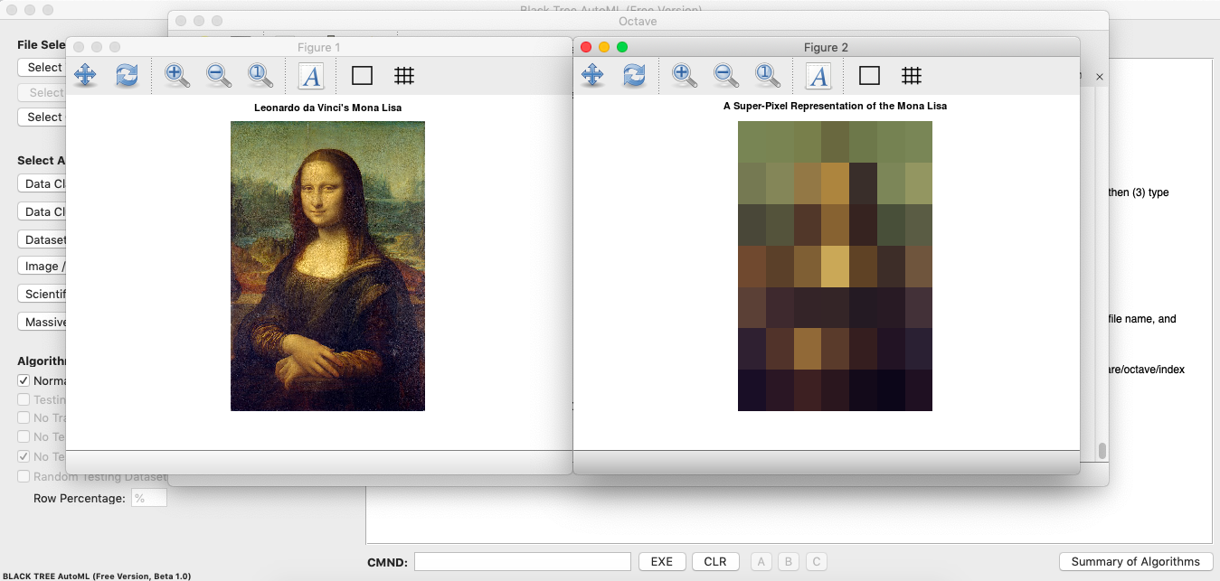
As noted, you cannot select the prediction algorithm, as it is automatically fixed to Supervised Delta Prediction for Image Classification. Moreover, you cannot select the image pre-processing algorithm, which is described in Section 1.3 of Vectorized Deep Learning, that generates super-pixel representations of each image in the dataset, thereby compressing them, allowing for extremely fast clustering and prediction. Finally, the images must be greyscale, and the dataset cannot contain more than 2,500 images. This will obviously not be the case for the Pro Version, which will include a wide variety of Image and Video Classification algorithms, with no limits on the number of rows or formats, or your ability to mix and match prediction and image pre-processing algorithms. The Free Version includes a teaser of RGB image processing, using a picture of Da Vinci’s Mona Lisa:
The teaser RGB image pre-processing demo, compressing The Mona Lisa into a super-pixel image with just 147 pixels, out of an original 2,110,464 pixels.
HOW DOES IT WORK?
The basic premise behind the software is that if a dataset is what I call locally consistent, then you can prove that the Nearest Neighbor algorithm will generate perfect accuracy (see, Analyzing Dataset Consistency, generally). In simple terms, a dataset is locally consistent if classifications don’t change over small distances. In practice, of course, datasets are not perfect, and what the algorithms attempt to do, is identify likely errors, ex ante, and “reject” them, leaving only the best predictions, which typically produces very high accuracies, and in the case of the Supervised Delta Prediction algorithm, nearly and at times actually perfect accuracies. The advantage of this approach over Neural Networks and other typical techniques, is that all of these algorithms have polynomial runtimes, and moreover, many of the processes can be executed in parallel, leading to what is at times almost instantaneous and highly accurate classifications and predictions, and in every case, radically more efficient processing than any approach to deep learning of which I am aware.
I have also developed specialized algorithms designed for thermodynamics, that can be applied to any massive Euclidean dataset, that allow for tens of millions of vectors to be classified and clustered in polynomial time (see Section 1.4 of Vectorized Deep Learning). These algorithms are of course not included in the Free Version, but will be included in the Pro Version, which again, is just $199 per user per year, or $1,000 for one user, for a lifetime commercial license. The Pro Version should be available in about a month from today.
I welcome feedback on the Free Version, particularly from Swift developers that have any insights, criticisms, tips, or questions, and you can reach me at [charles at BlackTreeAutoML dot com].
This code is included in my full library, but because it is so useful, I thought I would isolate it, in a command line script, which you can find on Research Gate.
Out of curiosity, I experimented with alternative normalization algorithms, and the results are basically the same as my core approach, which is to iterate through different digit scales, and run nearest neighbor, selecting the digit scale that generates the highest accuracy for nearest neighbor. The reason this works, is because you’re maximizing local consistency, by definition. The alternative approach, is to run a different algorithm, and test its accuracy, in this case, I ran a cluster prediction algorithm. Limited testing suggests it’s at best just as good, and possibly not as good, so given that nearest neighbor is incredibly fast when vectorized (i.e., O(number of rows)), there’s no practical reason to do otherwise.
You can find an example of the alternate code on Research Gate.
I am of course in the process of writing my AutoML Software, and I decided to include a supervised version of my modal prediction algorithm (not sure if it will be in the free version).
I was on a Meetup video conference, and someone mentioned a dataset that doesn’t cluster well (the UCI Sonar Dataset), so I naturally did a bit of work on it, and it turns out, the dataset literally contains very few clusters. Specifically, roughly 34% of the rows are contained in spherical clusters. The average cluster size over all rows is about .8 elements per cluster, again suggesting that you’re not going to get good clustering out of this dataset, because there are no real clusters to begin with, just as a matter of geometry. Nearest Neighbor nonetheless performs reasonably well, with an accuracy of 82.692%.
I’ve updated the “Magic Button” code to accommodate a training / testing structure, because I have to do it anyway at some point, when I release the Pro Version of my AutoML Software, Black Tree. It’s the same thing, the only difference is it draws the clusters from the training dataset, given the testing dataset, which keeps the wall up between the training and testing datasets.
Out of an abundance of caution, I’m incrementally uploading my work to DropBox, and so far I’ve included all of my recent scientific papers, and some of my music:
When you’re given a function, as observed, you will have discontinuity, and so the question becomes, is the discontinuity the result of observation, or the result of the underlying function itself? And in each case, how can I measure that, given my observed data, which is likely all you have to work with? It just dawned on me, my paper, “Sorting, Information, and Recursion“, seems to address exactly this topic. Specifically, Equation (2) will increase as the distance between the terms in a sequence increases. So as a result, what you can do is, first test the data using Equation (2) as is, without sorting the data. So for example, given , we would take the difference between adjacent range values as is, producing the vector . Then calculate using that vector. Then, you sort the range values, in this case producing , and repeat this, and the degree to which changes in the latter case, is a measure of how continuous your data is, because continuous data will have small gaps in the range values, and will be locally sorted in some order, as a consequence. Note that you should use the variant of Equation (2) I presented in Footnote 5, because for a continuous function, the distance between range values will likely be less than 1, and if you do that, then tighter and tighter observations will cause to get closer and closer to .
So I’m sure I shared it somewhere, though I’m not going to bother to look for it, I developed a method for finding the degree of a function (as a polynomial) using differentiation, the idea being that you differentiate numerically some fixed number of times (simply taking the difference between adjacent terms). Then you find the derivative that is closest to zero, by simply taking the sum over the terms. So for example, if you have range values (3,4,5), taking the difference between adjacent terms produces the vector (1,1), and doing that again you have (0). In the real world, data will not be so nice, but you can find the vector that is closest to zero by taking the sum over the vector. Now you know the next vector up is a linear function, the one after that second degree, and so on. Once you get back up to the function, now you know the degree of the function as a polynomial, and then you can use simple Gaussian Elimination to solve for the function as a polynomial. This algorithm will be included in the pro version of my AutoML software.
 plain text, CSV file, with integer classifier labels in column
  .
.
 , we would take the difference between adjacent range values as is, producing the vector
  . Then calculate
  using that vector. Then, you sort the range values, in this case producing
  , and repeat this, and the degree to which
  .
.