Introduction
I’m building up to a formal paper on human history that uses Machine Learning applied to mtDNA. You can find an informal but fairly rigorous summary that I wrote here [1], that includes the dataset in question and the code. In this note, I’m going to treat the topic at the individual genome level, whereas in [1], I generally applied algorithms to entire populations at a time (i.e., multiple genomes of the same ethnicity), and looked at genetic similarities across entire populations. The goal here is to tell the story of the Heidelbergensis maternal line, which is the largest maternal line in the dataset, accounting for 414 of the 644 genomes in the dataset (i.e., 62.35%). Specifically, 414 genomes are at least a 90% match to either Heidelbergensis itself, or one of the related genomes we’ll discuss below.
The Dataset
The dataset consists of 644 whole mtDNA genomes taken from the NIH database. There are therefore 644 rows, and 

I’ve diligenced the genome provenance files (see, e.g., this Norwegian genome’s provenance file) to ensure the ethnicity of the individual in question is, e.g., a person that is ethnically Norwegian, as opposed to a resident of Norway. The dataset consists of 75 classes of genomes, which are, generally speaking, ethnicities, and column N+1 contains an integer classifier for each genome, representing the ethnicity of the genome (e.g., Norway is represented by the classifier 7). The dataset also contains 19 archaic genomes, that similarly have unique classifiers, that are treated as ethnicities as a practical matter. For example, there are 8 Neanderthal genomes, each of which have a classifier of 32, and are for all statistical tests treated as a single ethnicity, though as I noted previously, Neanderthals are decidedly heterogenous. So big picture, we have 644 full mtDNA genomes, each stored as a row in a matrix (i.e., the dataset), where each of the first
Heidelbergensis and mtDNA
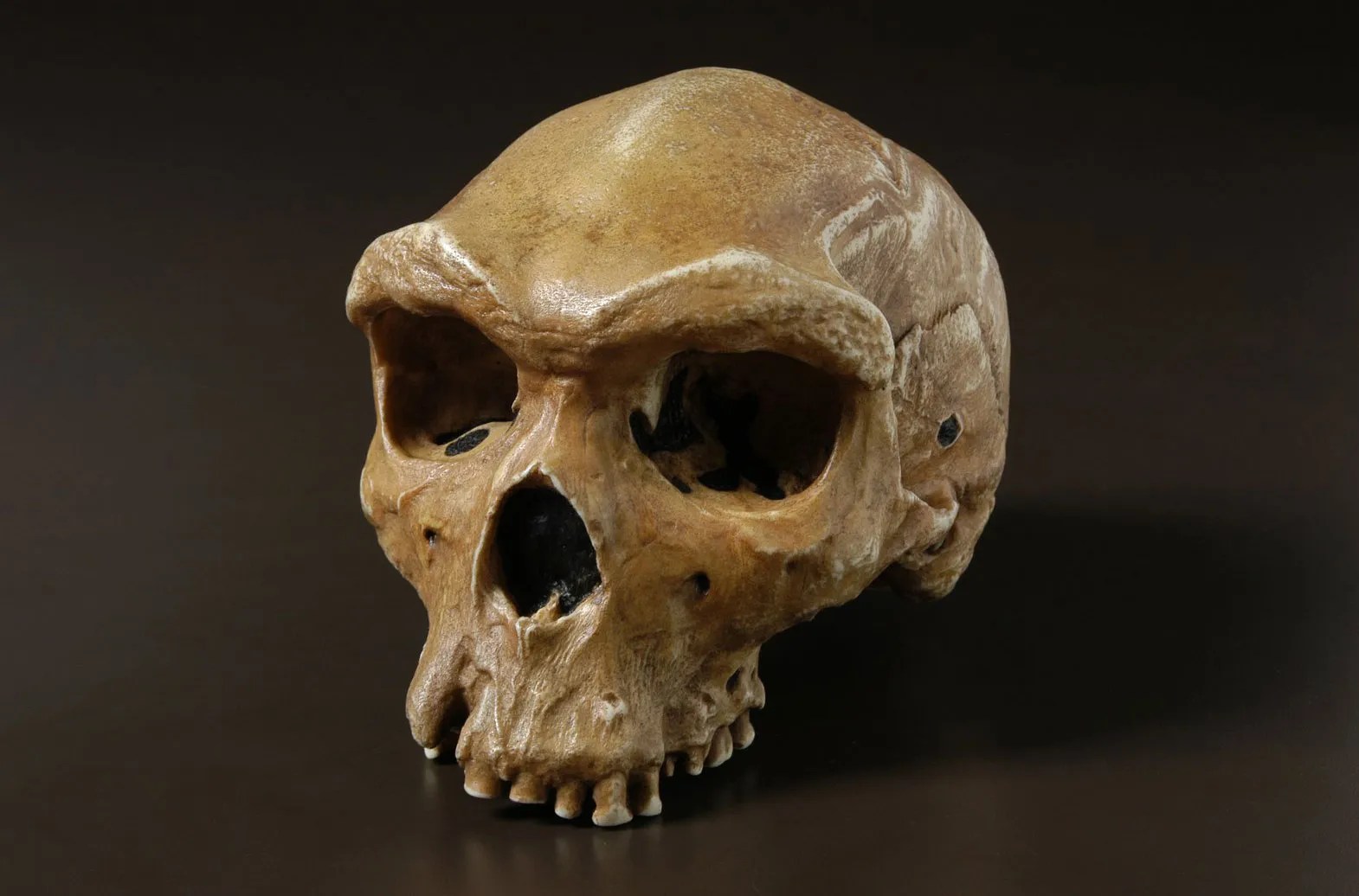
Heidelbergensis is an archaic human that lived (according to Brittanica) approximately 600,000 to 200,000 years ago. When I first started doing research into mtDNA, I immediately noticed that a lot of modern mtDNA genomes were a 95% or more match to Heidelbergensis. I thought at first I was doing something wrong, though I recently proved (both mathematically and empirically) that this is definitely not the case, and in fact, there’s only one way to compare whole mtDNA genomes. You can read the previous note linked to for details, but the short story is, mtDNA is generally inherited directly from your mother (i.e., there’s no paternal DNA at all in mtDNA), with no mutations, though mutations can occur over long periods of time (i.e., thousands of years, or sometimes more).
As a result, any method you use to compare an entire mtDNA genome must be able to produce nearly perfect matches, since a large enough dataset should contain a basically perfect match for a significant number of genomes, given mtDNA’s extremely slow rate of mutation. Said otherwise, if you have a large number of whole mtDNA genomes, there should be nearly perfect matches for a lot of the genomes in the dataset, since mtDNA mutates extremely slowly. There are of course exceptions, especially when you’re working with archaic genomes that might not have survived to the present, but the gist is, mtDNA mutates so slowly, someone should have basically the same mtDNA as you. Empirically, there’s exactly one method of whole-genome comparison that accomplishes this, which is explained in the previous link and contains the applicable code to test the hypothesis.
Just in case it’s not clear, whole-genome comparison means you take two entire genomes, and compare them side-by-side, rather than looking for individual sequential segments like genes, which until recently, was the more popular approach. If you’re curious, I’ve demonstrated that whole-genome comparison, and random base selection, are categorically superior to relying on sequential bases (e.g., genes) for imputation, at least as applied to mtDNA. See, A New Model of Computational Genomics [2]. We will also discuss using genome segments in the final section below.
Whole-Genome Comparison
The method of comparison that follows from this observation is straight forward, you simply count the number of matching bases between two genomes. So for example, if we’re given genome 


This makes whole-genome comparison super easy, and incredibly fast, and in fact, my software can compare a given genome to all 644 genomes in the dataset in just 0.02 seconds, running on an Apple M2 Pro, producing a ton of statistics for the input genome, not just the number of matching bases. Sure, it’s a great machine, but it’s not a super computer, which means now everyone can do real genetic analysis on consumer devices. Once popularized, these methods will probably make short work of the complete history of mankind, and possibly the entire history of life itself, since mtDNA is not unique to humans. Further, these methods and their results are rock solid, empirical evidence for the Theory of Evolution, which as you’ll see below, is not subject to serious criticism, at least with respect to mtDNA.
Modern Relatives of Heidelbergensis
As noted above, many modern living humans have mtDNA that is a 95% or more match to the single Heidelbergensis genome in the dataset. The genome was found at Sima de Los Huesos, and there is apparently some debate about whether it is actually a Neanderthal, but it is in all cases a very archaic genome from around 500,000 years ago. As such, though I concede this Heidelbergensis genome is a 95.10% match to the third Neanderthal genome in my dataset, which is from around 100,000 years ago, I think it’s best to distinguish between the two, given the huge amount of time between the two genomes, and the fact that they’re not exactly the same genome.
Recall that we are comparing whole-genomes by simply counting the number of matching bases, which we’ll call the match count. We can therefore, set a minimum match count of say 
The plain takeaway is that many modern humans carry mtDNA that is close to Heidelbergensis, peaking at a 96.69% match for a Kazakh individual. As noted above, when working with modern genomes, you’ll often find a basically perfect match that exceeds 99%, but when working with archaic genomes, that’s not always the case, and it makes perfect sense, since so much time has elapsed, that even with the incredibly slow rate of mutation for mtDNA, a few percentage points of mutation drift is to be expected.
The Phoenician People
The Phoenicians were a Mediterranean people that existed from around 2500 BC to 64 AD. Though there could be other example genomes, the Phoenicians are a great case study because they are a partial match to Heidelbergensis, and a partial match to the Pre-Roman Ancient Egyptian genome. You can already appreciate the intuition, that Heidelbergensis evolved into the Phoenicians, and then the Phoenicians evolved further into the Ancient Egyptians.
Now the real story is more complicated, and it doesn’t look like all of this happened in the Mediterranean. Instead, it looks like human life begins in West Africa, migrates to roughly the Mediterranean and Eurasia, migrates further to somewhere around Northern India, and then spreads back to Europe and Africa, and further out into East Asia. You can read [2] for more on this topic, this note will instead be focused on the evolution of the individual genomes, and less so on claims regarding their historical geographies. That is, I’m going to present you with a set of genomes that begin with Heidelbergensis, and end in the Icelandic people, who are almost certainly Vikings, but I’m not going to argue too much about where these mutations happened, outside of a few notes for context, so that it’s not all happening in a void.
Returning to the Phoenicians, we want to show first, that the Phoenicians evolved from Heidelbergensis. All of these steps will involve epistemological reflections, so that we can be comfortable that we’re asserting reasonable claims. That said, as you’ll see, all of these claims are uncertain, and plainly subject to falsification, but that’s science. To begin, note that there are 6 Phoenician genomes in the dataset, and that the first Phoenician genome in the dataset (row 415) is at least a 99.72% match to the other 5 Phoenician genomes. As such, to keep things simple, we will treat this first Phoenician genome as a representative genome for the entire class of Phoenicians. Further, note that the first Phoenician genome is a 41.17% match to Heidelbergensis. If we were comparing two random genomes, then the expected match count is 25% of the genome, since the distribution is given by the Binomial Distribution, with a probability of success of 

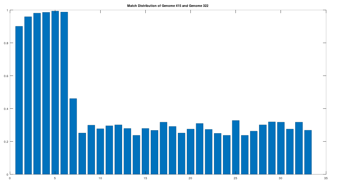
The claim that the two genomes are truly related finds further support in the location of the matching bases, which are concentrated in the first 3,500 bases, which is shown in the chart below. The chart below is produced by taking 500 bases at a time, starting with the first 500 bases of each genome, and counting how many bases within that 500-base segment match between the two genomes. The maximum match count is of course 500 bases, which would produce a height of 1.0, or 100%. This process continues over the entire genomes, producing the chart below. As you can see, the most significant matches are clustered in the first 7 segments, representing the first 3,500 bases of the genomes. The argument is, because there is a significant, contiguous segment within the genomes that are highly similar, we can confidently rule out chance as the driver of the similarity. You can never be totally certain, but since it’s probably not chance that’s driving the similarity, the logical conclusion is that heredity and mutation is what caused the similarity between the two genomes. Now we don’t know the direction of time from this analysis alone (i.e., either genome could have evolved into the other), but because Heidelbergensis is very archaic, the logical conclusion, is that Heidelbergensis mutated, eventually forming the Phoenician maternal line.
One important point to note, is that even if a genome evolves, it does not imply that all instances of that genome evolve. For example, as noted above, 100% of the living Iberian Romani people are at least a 90% match to Heidelbergensis, demonstrating that at least some Heidelbergensis genomes did not evolve into the Phoenician line, and instead remained roughly the same over time. As such, we can say confidently that mtDNA is very slow to mutate as a general matter, but the rates of mutation are heterogenous.
Just to close this section with some context for modern humans that carry the Phoenician line, 80% of living Sardinians and 33.33% of living Vedda Aboriginals are at least a 90% match to the Phoenicians. Obviously, it’s a bit shocking that you’d have Phoenician mtDNA in Asia, but if you read [2], you’ll quickly learn that these are global maternal lines that often contain multiple disparate people. Two common sense explanations, (1) the Phoenicians really made it to Asia or (2) there’s a common ancestor for both the Phoenician and Vedda people, presumably somewhere in Asia. Hypothesis (2) finds support in the fact that 10.52% of Mongolians are also at least a 90% match to the Phoenicians. This is a complicated topic, and it’s just for context, the real point of this note is that you can plainly see that Heidelbergensis evolved, which is already interesting and compelling evidence for the Theory of Evolution, and specifically, it evolved into the Phoenician maternal line.
The Ancient Egyptians
Introduction
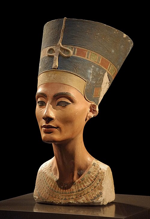
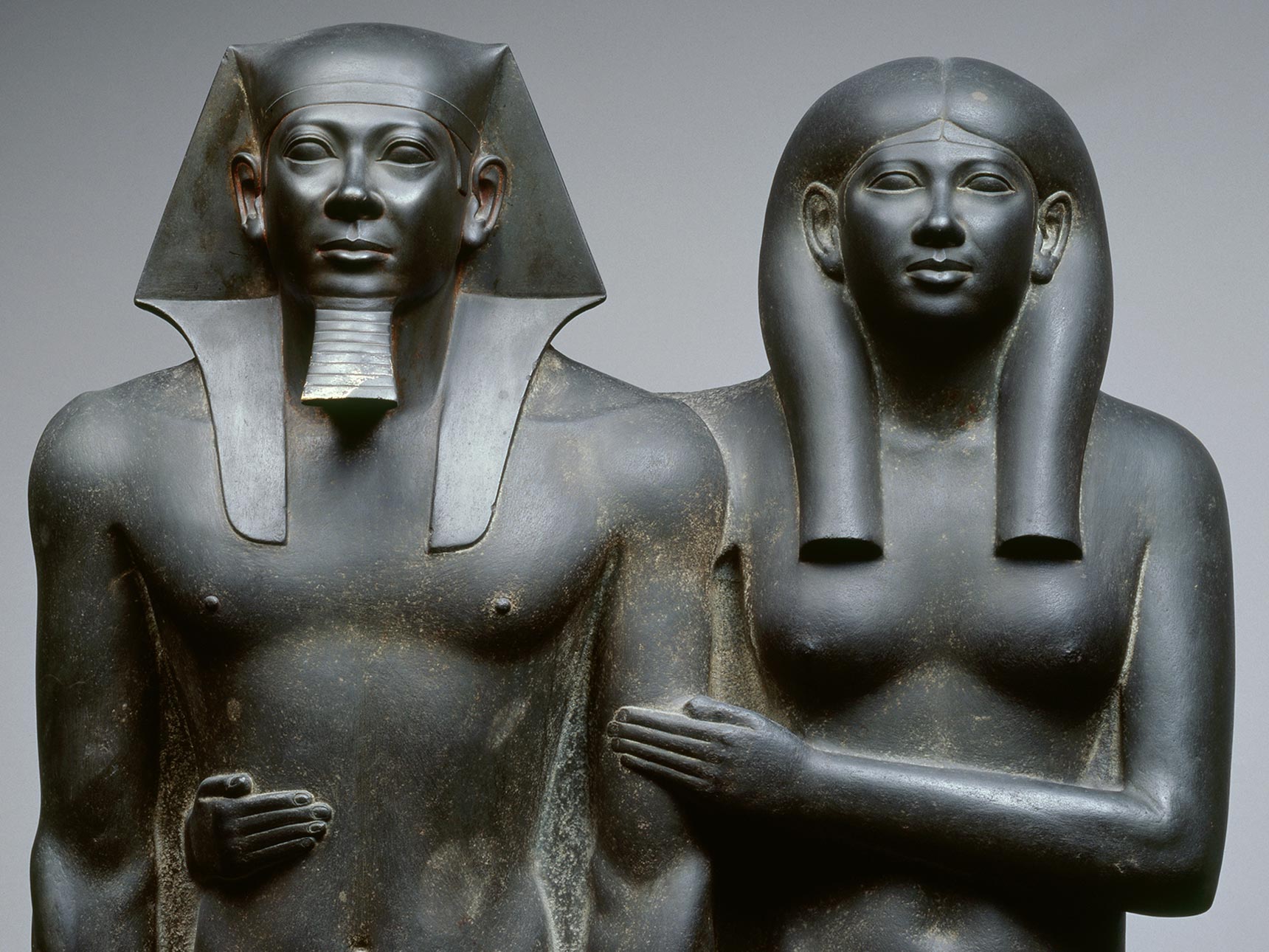
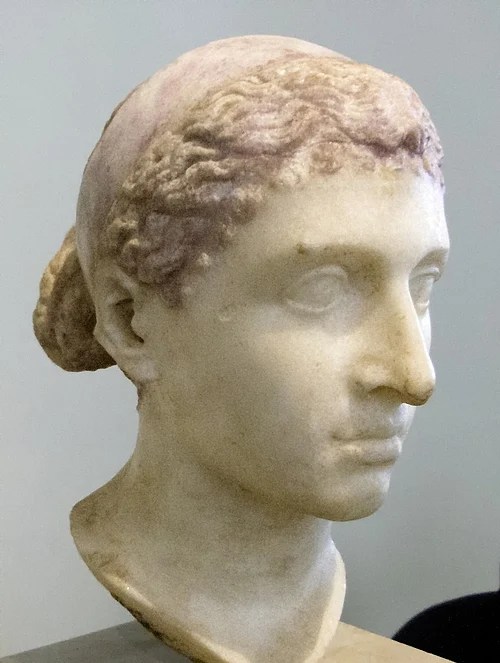
The Ancient Egyptians were a Mediterranean civilization that lasted from around 3150 BC to 30 BC, until it was ruled by Rome, from around 30 BC to 642 AD. There are two Ancient Egyptian genomes in the dataset, one from approximately 2000 BC, before Roman rule, and another genome from approximately 129 to 385 AD, during Roman rule. This is a huge amount of time, and so it’s not surprising that the demographics changed. But the Ancient Egyptians present a shocking demographic shift, from earlier rulers that were plainly of Asian origin, to rulers that looked, and were known to be, European. For example, see the panel of images below, with Nefertiti (1353 to 1336 BC) on the left, then King Menkaure and his Queen (2550 BC to 2503 BC), and finally Cleopatra (51 to 30 BC) on the right, who is known to be Macedonian.
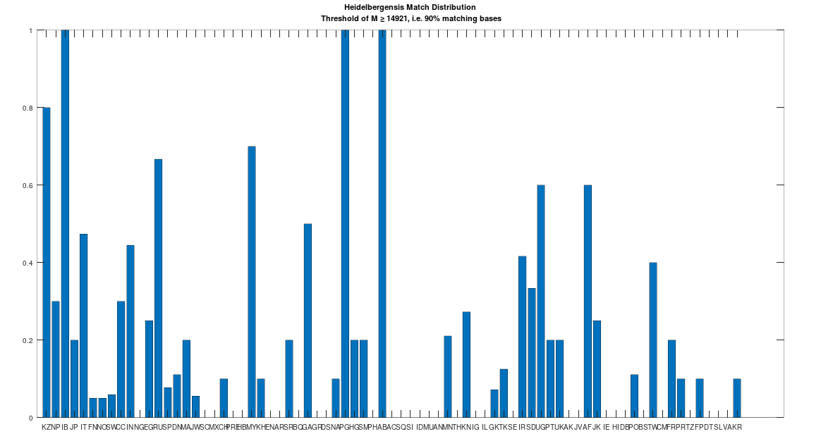
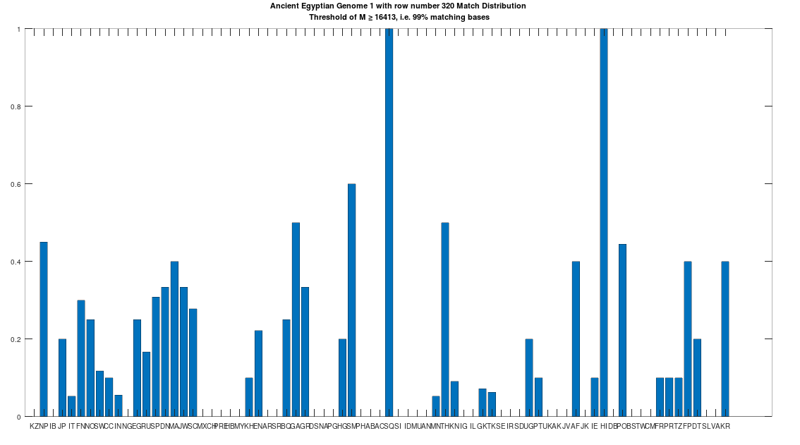
The hypothesis that the earlier Egyptians were of Asian origin is further supported by the chart below, which shows the distribution of genomes that are at least a 99% match to the Pre-Roman Egyptian genome. The full set of population acronyms are in [2], but for now note that NP stands for Nepal, JP stands for Japan, FN stands for Finland, NO stands for Norway, EG stands for modern day Egypt, DN stands for Denmark, GA stands for Georgia, TH stands for Thailand, FP stands for Philippines, and KR stands for Korea. As you can plainly see, the Pre-Roman Egyptian genome is very common in Northern Europe and East Asia, with very little representation in Africa outside of modern day Egypt, though there is some nuance to this. See [2] for more. The point is, the Pre-Roman Egyptian genome probably comes from Asia, and spread to Northern Europe, North Africa, and East Asia, and as far as I know, this is not exactly accepted history, but it’s clearly the case.
Ancestry from Heidelbergensis and Phoenicia
As noted above, the Pre-Roman Egyptian genome (row 320) is a partial match to the Phoenician genome, with a match count of 88% of the genome. This is obviously very high, so we can be confident that this is not the result of chance, and is instead the result of heredity and mutation. Further, because we have assumed that Heidelbergensis is the ancestor of the Phoenician genome (since it is archaic), it cannot be the case that the Ancient Egyptian genome is also the ancestor of the Phoenician genome. Specifically, because mtDNA is inherited directly from the mother to its offspring, there can be only one ancestral maternal line for a given genome, though there can be intermediate ancestors. For example, genome A mutates into genome B, which in turn mutates into genome C. However, because the Ancient Egyptian genome has a match count of 29.73% to Heidelbergensis, the Ancient Egyptian genome cannot credibly be an intermediate ancestor of the Phoenicians, between Heidelbergensis and the Ancient Egyptians. Therefore, it must be the case, given our assumption that Heidelbergensis is the ancestor of the Phoenicians, that the Pre-Roman Ancient Egyptian genome is the descendant of the Phoenicians.
Historically, this is counterintuitive, because the Ancient Egyptians are more ancient than the Phoenicians, but as noted above, these maternal lines are broader groups, I’m simply labelling them by using the most famous civilizations that have the genomes in question. Further, as noted above, a lot of this evolution probably happened in Asia, not the Mediterranean. So one sensible hypothesis is that Heidelbergensis travelled East, mutated to the Phoenician line somewhere in Asia, and then that Phoenician line mutated further into the Pre-Roman Ancient Egyptian line, again probably somewhere in Asia. This is consistent with the fact that 76.67% of Kazakh genomes, 44.44% of Indian genomes, and 66.67% of Russian genomes are at least a 95% match to Heidelbergensis, making it plain that Heidelbergensis travelled to Eurasia and Asia. In contrast, as noted above, the Pre-Roman Ancient Egyptian line is found generally in Northern Europe, East Asia, and North Africa, consistent with a further migration from Eurasia and Asia, into those regions.
The Roman Era Egyptian Genome
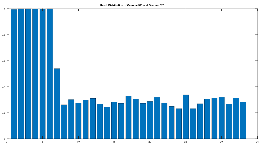
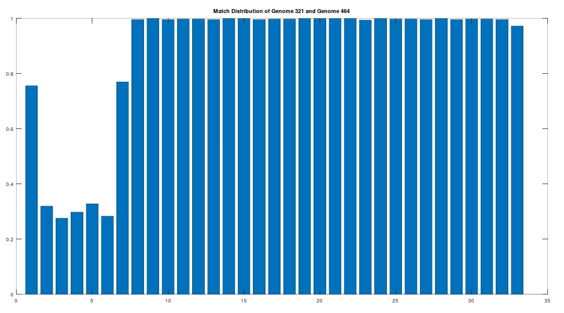
As noted above, the Ancient Egyptians were ruled by Rome from around 30 BC to 642 AD. Though it is reasonable to assume that there were resultant demographic changes, we’re only looking at two genomes from Ancient Egypt, and so the point is not that these two genomes are evidence of that demographic change. The evidence of the demographic changes are above, in the form of archeological evidence of completely different people ruling their civilization. The point of this section is instead that there is a second genome that was found in Egypt, that is dated to around 129 to 385 AD, squarely during Rome’s rule over Egypt, that is related to the other Ancient Egyptian genome discussed above. Specifically, the Roman Era Egyptian genome (row 321) is a 42.20% match to the Pre-Roman Egyptian genome (row 320). Now, that is significantly above chance (i.e., 25%), but we can also perform the same analysis we did above, looking to 500-base segments for confirmation that the match count is not the result of chance, which is shown below. Again, the most similar regions are concentrated in the first seven, 500-base segments, plainly suggesting heredity rather than chance.
Because we have assumed the Phoenician genome is the ancestor of the Pre-Roman Egyptian genome, it cannot be the case that the Roman Era Egyptian genome is the ancestor of the Pre-Roman Egyptian genome. We can further rule out the possibility of an intermediate relationship by noting that the match count between the Roman Era Egyptian genome and the Phoenician genome is 30.50%. Therefore, we have established a credible claim that Heidelbergensis evolved into the Phoenician maternal line, which in turn evolved into the Pre-Roman Egyptian maternal line, and then further into the Roman Era Egyptian maternal line.
Iceland and the Vikings
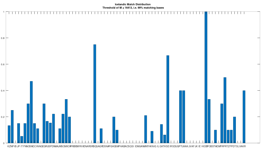
The dataset contains a single Icelandic genome, though it was collected from a person in Canada. So it’s fair to express some skepticism, as people can deliberately deceive researchers, though I’m not sure why you would. But that said, let’s kick the tires, and see what populations are at least a 99% match to this purportedly Icelandic genome, which is shown in the chart below. Because these genomes are members of large global groups, we need to be careful in this type of analysis, and accept uncertainty. But you can plainly see in the chart below, that the genome in question is a pronounced match to Sweden (SW) and Norway (NO). Further, the Icelandic genome is a 99.77% match to the single Dublin genome (DB), and Dublin was a Viking colony. Now all of this is subject to falsification and uncertainty, but I think we can be reasonably confident, that the person in question really is of Icelandic ancestry.
With that, we can turn to heredity, in particular noting that the Roman Era Egyptian genome is an 87.79% match to the Icelandic genome. Though that is an extremely high match count, that cannot credibly be the result of chance, we can also examine the structure of the matching segments, just as we did above, since we have some doubt regarding the provenance, given that the individual lived in Canada. This is shown below, and as you can see, it is plainly not the result of chance, since the vast majority of matching segments are from and including segment 7 onward. Because we have assumed that the Pre-Roman Egyptian genome is the ancestor of the Roman Era Egyptian genome, it cannot be the case that the Icelandic genome is the ancestor of the Roman Era Egyptian genome. To rule out an intermediate relationship, we can simply note that the match count between the Icelandic genome and the Pre-Roman Egyptian genome is 30.29%. Therefore, we have put together a credible claim that Heidelbergensis evolved into the Phoenician maternal line, which in turn produced the Pre-Roman Egyptian maternal line, then the Roman Era Egyptian maternal line, and finally, the Icelandic maternal line. Because Iceland was uninhabited before the Vikings, it is reasonable to assume that the Icelandic genome was included in the set of Viking maternal lines.
Measuring Genetic Drift
As you can see, whole-genome comparison is nothing short of amazing, allowing us to build rock solid arguments regarding the history of mankind, and demonstrating plainly the Theory of Evolution is real. That said, if a genome is subject to what’s called an indel, which is an insertion or deletion, then the match count between two genomes will generally drop to around 25%, i.e., chance. As a simple example, consider genomes 


As a result, geneticists make use of what are called local alignments, which take segments from one genome, and find the best match for that segment in the comparison genome. Continuing with 


Applying this to the narrative above, we can run the local alignment algorithm comparing Heidelbergensis to the Icelandic genome. This produces a match count of 15,908, and therefore, 
 and
and  , respectively. Let’s further assume that we are surrounded almost exclusively by positive mass, which again is denoted by
  to represent a photon, we could write that
  , to represent a positron and electron colliding to form a photon. Similarly, we could write that
  to represent a light on light collision producing an electron-positron pair.
 and
and  . The question is, what do we get when we combine the negative-mass versions of an electron and positron? Expressed symbolically,
  , where
  , as a particle distinct from ordinary light. Specifically, if we further posit that negative-mass light does not interact with positive mass, and that positive-mass light (our ordinary photons) do not interact with negative mass, then that negative mass would not be detectable using ordinary photons. Ironically, this is a kind of “dark” matter, but it’s not the nonsense hypothesized hitherto.
 and
and  . If we count matching bases using the first index of each genome, then the number of matching bases is zero. If instead we start at the first index of
  and the second index of
  (and loop back around to the first ‘G’ of
  and
and  . First you’ll note these genomes are not the same length, unlike in the example above, which is another factor to be considered when developing an alignment for comparison. If we simply use the first three bases of each genome for comparison, then the match count will be one, since the first two initial ‘A’s match. If instead we use index two of
  , then the entire
  sequence matches, and the resultant match count will be three.
 . As for accuracy, using Nearest Neighbor to predict the ethnicity of each individual in my dataset produces an accuracy of 30.87%, and because there are 75 global ethnicities, chance implies an accuracy of
  . As such, we can conclude that the Nearest Neighbor algorithm is not producing random results, and more generally, produces results that provide meaningful information about the ethnicities of individuals based solely upon their mtDNA, which is remarkable, since ethnicity is a complex trait, that clearly should depend upon paternal ancestry as well.
 of Norwegian genomes map to Pashtuns, who are
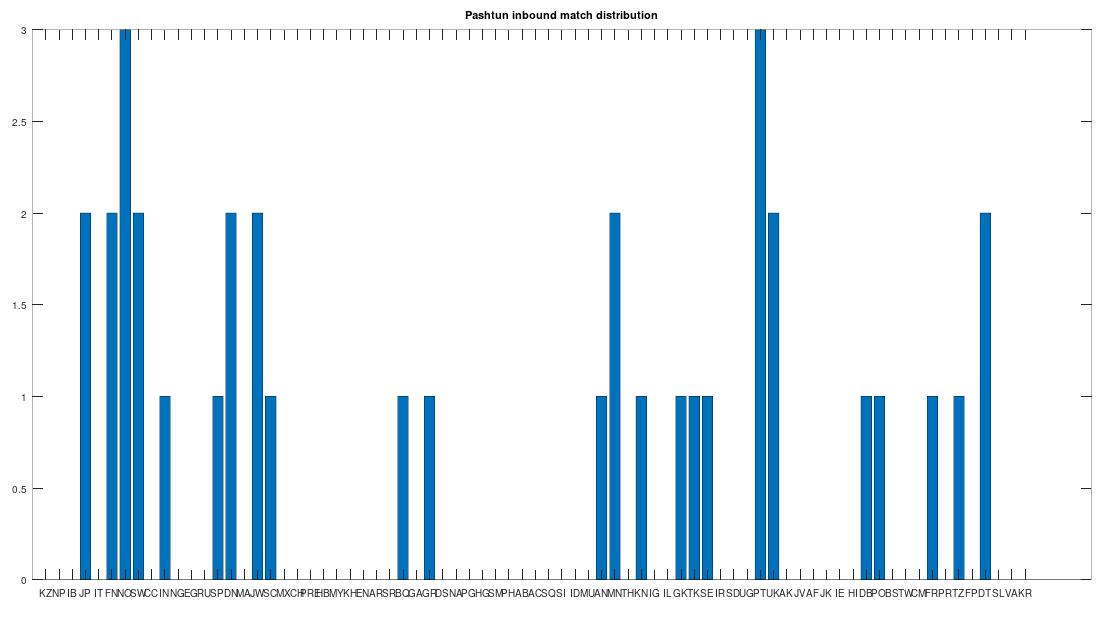
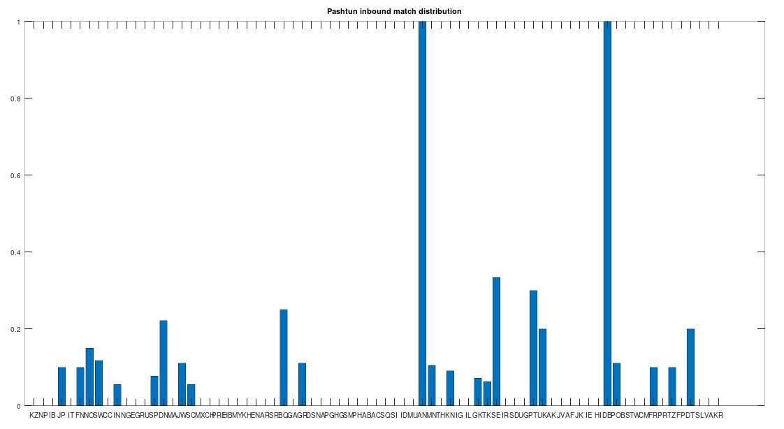
 , so these are plainly meaningful, nearly identical matches. Finally, these Pashtun genomes that are turning up as Nearest Neighbors are heterogeneous. That is, it’s not the case that a single Pashtun genome is popping up globally, and instead, multiple distinct Pashtun genomes are popping up globally as Nearest Neighbors. One not-so-plausible explanation that I think should be addressed is the