The Demand For Risk And A Macroeconomic Theory of Credit Default Swaps: Part 2

January 10, 2009March 12, 2023 / erdosfan / 38 Comments

Redux And Reduction

In the previous article, we defined a highly abstract framework that considered the subjective expected payout of both sides of a fixed fee derivative. In this article, we will apply that model to the context of credit default swaps and will show that the presence of credit default swaps and synthetic bonds should be expected to reduce the demand for “real” bonds (as opposed to synthetic bonds) and thereby reduce the net exposure of an economy to credit risk.

The Demand For Credit Default Swaps

In the previous article, we plotted the expected payout of each party to a credit default swap as a function of the fee and each party’s subjective valuation of the probability that a default will occur. The simple observation gleaned from that chart was that if we fix the subjective probabilities of default, protection sellers expect to earn more as the price of protection increases and protection buyers expect to earn more as the price of protection decreases. Thus, as the the price of protection increases, we would expect protection seller side “demand” to increase and expect protection buyer side “demand” to decrease. But how can demand be expressed in the context of a credit derivative? The general idea is to assume that holding all other variables constant, the size of the desired notional amount of the CDS will vary with price. So in the case of protection sellers, the greater the price of protection, the greater the notional amount desired by any protection seller.

In order to further formalize this concept, we should consider each reference entity as defining a unique demand curve for each market participant. We should also distinguish between demand for buying protection and demand for selling protection. For convenience’s sake, we will refer to the demand for selling protection as the supply of credit protection and demand for buying credit protection as the demand for credit protection. For example, consider protection seller X’s supply curve and protection buyer Y’s demand curve for CDSs naming ABC as a reference entity. The following chart expresses the total notional amount of all CDSs desired by X and Y as a function of the price of protection.

supply-demand-credit-exposure1

As the price of protection approaches zero, Y’s desired notional amount should approach infinity, since at zero, Y is getting free protection and should desire an unbounded “quantity” of credit protection. The same is true for X as the price of protection approaches infinity.

Synthetic Bonds As Competing Goods With “Real” Bonds

Imagine a world without credit derivatives and therefore without synthetic bonds. In that world, there will be a demand curve for real ABC bonds as a function of the spread the bonds pay over the risk free rate, holding all over variables constant. Now imagine that credit default swaps were introduced to this world. We know that the cash flows of any bond can be synthesized using Treasuries and credit default swaps. For example, assume we have synthesized the cash flows of ABC’s bonds using the method described here. We would expect at least some investors to be indifferent between real ABC bonds and synthetic ABC bonds, since they both produce the same cash flows. Thus, the two are competing products in the sense that investors in real ABC bonds should be potential investors in synthetic ABC bonds. So because some investors will be indifferent between synthetic ABC bonds and real ABC bonds, synthetic ABC bonds will siphon some of the cash that would have otherwise gone to real ABC bonds. Thus, in a world with credit derivatives, we would expect there to be less demand for real bonds than would be present without credit derivatives. In the following chart we express the macroeconomic demand for real ABC bonds in terms of the spread over the risk free rate and the total par value desired by the market.

demand-with-credit-derivatives

Thus, the demand for credit derivatives diminishes the demand for real bonds. Although we cannot know exactly what the effect on the demand curve for real bonds will be, we can safely assume that it will be diminished at all levels of return, since at each level, at least some investors will be indifferent to real bonds and synthetic bonds, since each offers the same return.

Real Cash Losses Versus Wealth Transfers Through Derivatives

Economics already has a term to describe payouts under credit default swaps: wealth transfers. Although ordinarily used to describe the cash flows of tax regimes, the term applies equally to the payments under a credit default swap. As described in the previous article, there are no net cash losses under a credit default swap. There is a payment of money from one party to another, the net effect of which is a wealth transfer. That is, credit default swaps, like all derivatives, simply rearrange the current allocation of cash in the financial system, and nothing is lost in process (ignoring transaction costs, which are not relevant to this discussion).

When a real bond defaults, a net cash loss occurs. The borrower has taken the money lent to it by investors, lost it, and the investors are not fully paid back. Therefore, both the borrower and the investors incur a cash loss, creating a net cash loss to the economy. So, in the case of a synthetic ABC bond, upon the default of one of ABC’s bonds, a wealth transfer occurs from the protection seller to the protection buyer and the net effect is null. In the case of a real ABC bond, upon the default of that bond, the investors will lose some of their principle and ABC has already lost some of the money it was lent, the net effect of which is a loss to the economy.

So every dollar siphoned away from real bonds by synthetic bonds is a dollar that will not be lost in the economy upon the occurrence of a credit event. If there were no credit derivatives, then that dollar would have been invested in real bonds and thereby lost upon the occurrence of a credit event. Therefore, the net losses to the economy upon the occurrence of a credit event is less with credit derivatives than without. In the following diagram, the two circles of each transaction represent the parties to that transaction. In the case of real bonds, one of the parties is ABC and the other is an investor. In the case of synthetic bonds, one is the protection seller and the other is the protection buyer of the credit default swap underlying the synthetic bond.

net-losses-with-derivatives

This diagram simply demonstrates what was described above. Namely, that with credit derivatives, some investors will choose synthetic bonds rather than real bonds, thereby reducing the amount of cash exposed to credit risk. Thus, rather than increase the impact of credit risk, credit default swaps actually decrease the impact of credit risk by placating the demand for exposure to credit risk with synthetic instruments that are incapable of producing net losses. However, there may be consequences arising from credit default swaps that cause actual cash losses to an economy, such as a firm failing because of its obligations under credit default swaps. But the failure is not caused by the instrument itself. The nature of the instrument is to reduce the impact of credit risk. The firm’s failure is caused by that firm’s own poor risk management.

The Demand For Risk And A Macroeconomic Theory of Credit Default Swaps: Part 1

December 18, 2008March 12, 2023 / erdosfan / 15 Comments

A Higher Plane

In this article, I will return to the ideas proposed in my article entitled, “A Conceptual Framework For Analyzing Systemic Risk,” and once again take a macro view of the role that derivatives play in the financial system and the broader economy. In that article, I said the following:

“Practically speaking, there is a limit to the amount of risk that can be created using derivatives. This limit exists for a very simple reason: the contracts are voluntary, and so if no one is willing to be exposed to a particular risk, it will not be created and assigned through a derivative. Like most market participants, derivatives traders are not in engaged in an altruistic endeavor. As a result, we should not expect them to engage in activities that they don’t expect to be profitable. Therefore, we can be reasonably certain that the derivatives market will create only as much risk as its participants expect to be profitable.”

The idea implicit in the above paragraph is that there is a level of demand for exposure to risk. By further formalizing this concept, I will show that if we treat exposure to risk as a good, subject to the observed law of supply and demand, then credit default swaps should not create any more exposure to risk in an economy than would be present otherwise and that credit default swaps should be expected to reduce the net amount of exposure to risk. This first article is devoted to formalizing the concept of the price for exposure to risk and the expected payout of a derivative as a function of that price.

Derivatives And Symmetrical Exposure To Risk

As stated here, my own view is that risk is a concept that has two components: (i) the occurrence of an event and (ii) a magnitude associated with that event. This allows us to ask two questions: What is the probability of the event occurring? And if it occurs, what is the expected value of its associated magnitude? We say that P is exposed to a given risk if P expects to incur a gain/loss if the risk-event occurs. We say that P has positive exposure if P expects to incur a gain if the risk-event occurs; and that P has negative exposure if P expects to incur a loss if the risk-event occurs.

Exposure to any risk assigned through a derivative contract will create positive exposure to that risk for one party and negative exposure for the other. Moreover the magnitudes of each party’s exposure will be equal in absolute value. This is a consequence of the fact that derivatives contracts cause payments to be made by one party to the other upon the occurrence of predefined events. Thus, if one party gains X, the other loses X. And so exposure under the derivative is perfectly symmetrical. Note that this is true even if a counterparty fails to pay as promised. This is because there is no initial principle “investment” in a derivative. So if one party defaults on a payment under a derivative, there is no cash “loss” to the non-defaulting party. That said, there could be substantial reliance losses. For example, you expect to receive a $100 million credit default swap payment from XYZ, and as a result, you go out and buy $1,000 alligator skin boots, only to find that XYZ is bankrupt and unable to pay as promised. So, while there would be no cash loss, you could have relied on the payments and planned around them, causing you to incur obligations you can no longer afford. Additionally, you could have reported the income in an accounting statement, and when the cash fails to appear, you would be forced to “write-down” the amount and take a paper loss. However, the derivatives market is full of very bright people who have already considered counterparty risk, and the matter is dealt with through the dynamic posting of collateral over the life of the agreement, which limits each party’s ability to simply cut and run. As a result, we will consider only cash losses and gains for the remainder of this article.

The Price Of Exposure To Risk

Although parties to a derivative contract do not “buy” anything in the traditional sense of exchanging cash for goods or services, they are expressing a desire to be exposed to certain risks. Since the exposure of each party to a derivative is equal in magnitude but opposite in sign, one party is expressing a desire for exposure to the occurrence of an event while the other is expressing a desire for exposure to the non-occurrence of that event. There will be a price for exposure. That is, in order to convince someone to pay you $1 upon the occurrence of event E, that other person will ask for some percentage of $1, which we will call the fee. Note that as expressed, the fee is fixed. So we are considering only those derivatives for which the contingent payout amounts are fixed at the outset of the transaction. For example, a credit default swap that calls for physical delivery fits into this category. As this fee increases, the payout shrinks for the party with positive exposure to the event. For example, if the fee is $1 for every dollar of positive exposure, then even if the event occurs, the party with positive exposure’s payments will net to zero.

This method of analysis makes it difficult to think in terms of a fee for positive exposure to the event not occurring (the other side of the trade). We reconcile this by assuming that only one payment is made under every contract, upon termination. For example, assume that A is positively exposed to E occurring and that B is negatively exposed to E occurring. Upon termination, either E occurred prior to termination or it did not.

sym-exposure2

If E did occur, then B would pay $N \cdot(1 - F)$ to A, where F is the fee and N is the total amount of A’s exposure, which in the case of a swap would be the notional amount of the contract. If E did not occur, then A would pay $N\cdot F$ . If E is the event “ABC defaults on its bonds,” then A and B have entered into a credit default swap where A is short on ABC bonds and B is long. Thus, we can think in terms of a unified price for both sides of the trade and consider how the expected payout for each side of the trade changes as that price changes.

Expected Payout As A Function Of Price

As mentioned above, the contingent payouts to the parties are a function of the fee. This fee is in turn a function of each party’s subjective valuation of the probability that E will actually occur. For example, if A thinks that E will occur with a probability of $\frac{1}{2}$ , then A will accept any fee less than .5 since A’s subjective expected payout under that assumption is $N (\frac{1}{2}(1 - F) - \frac{1}{2}F ) = N (\frac{1}{2} - F)$ . If B thinks that E will occur with a probability of $\frac {1}{4}$ , then B will accept any fee greater than .25 since his expected payout is $N (\frac{3}{4} F - \frac{1}{4}(1 - F)) = N (F - \frac{1}{4} )$ . Thus, A and B have a bargaining range between .25 and .5. And because each perceives the trade to have a positive payout upon termination within that bargaining range, they will transact. Unfortunately for one of them, only one of them is correct. After many such transactions occur, market participants might choose to report the fees at which they transact. This allows C and D to reference the fee at which the A-B transaction occurred. This process repeats itself and eventually market prices will develop.

Assume that A and B think the probability of E occurring is $p_A$ and $p_B$ respectively. If A has positive exposure and B has negative, then in general the subjective expected payouts for A and B are $N (p_A - F)$ and $N ( F - p_B)$ respectively. If we plot the expected payout as a function of F, we get the following:

payout-v-fee4

The red line indicates the bargaining range. Thus, we can describe each participant’s expected payout in terms of the fee charged for exposure. This will allow us to compare the returns on fixed fee derivatives to other financial assets, and ultimately plot a demand curve for fixed fee derivatives as a function of their price.

A Conceptual Framework For Analyzing Systemic Risk

November 8, 2008March 11, 2019 / erdosfan / 20 Comments

The Cart Before The Horse

There has been a lot of chatter about the systemic risks posed by derivatives, particularly credit default swaps. Rather than offer any formal method of evaluating an enormously complicated question, pundits wield exclamation points and false inferences to distract from the glaring holes in their logic. Below I will not offer any definite answers to any questions about the systemic risks posed by derivatives. Rather, I will describe what I think is a reasonable and useful framework for analyzing systemic risks posed by derivatives. Unfortunately for some, this will involve the use of mathematics. And while the math used is fairly elementary, the concepts are not. This is especially true of the last section. That said, even if you do not fully understand the entirety of this article, one thing should be clear: questions about systemic risk are complex and anyone who gives declarative answers to such questions is almost certain to have no idea what they are talking about.

Risk Magnification And Syndication

As discussed here, derivatives operate by creating and allocating risks that did not exist before the two parties entered into the transaction. That is an unavoidable fact. Moreover, there is no physical limit to the notional amount of any given contract or the number of derivative contracts that parties can enter into. It is entirely up to them. That said, derivatives can be used to negate risks that parties were already exposed to in exchange for assuming other risks, thereby acting as a risk-switching/risk-transferring device. So, a corollary of these observations is that derivatives could be used to create unlimited amounts of risk but through that risk creation they could be used to negate an unlimited amount of risk that parties are already exposed to and thereby effectively “transfer” an unlimited amount of risk to those willing to be exposed to it.

Practically speaking, there is a limit to the amount of risk that can be created using derivatives. This limit exists for a very simple reason: the contracts are voluntary, and so if no one is willing to be exposed to a particular risk, it will not be created and assigned through a derivative. Like most market participants, derivatives traders are not in engaged in an altruistic endeavor. As a result, we should not expect them to engage in activities that they don’t expect to be profitable. Therefore, we can be reasonably certain that the derivatives market will create only as much risk as its participants expect to be profitable. Whether their expectations are correct is an entirely different matter, and any criticism on that front is not unique to derivatives traders. Rather, the problem of flawed expectations permeates all of human decision making.

Even if we ignore the practical limits to the creation of risk, derivatives allow for unlimited syndication of risk. That is, there is no smallest unit of risk that can be transferred. Consequently, any fixed amount of risk can be syndicated out to an arbitrarily large number of parties, thereby minimizing the probability that any individual market participant will fail as a result of that risk.

Finally, we should ask ourselves, what does the term systemic risk even mean? The only thing it can mean in the context of derivatives is that the obligations created by two parties will have an effect on at least one other third party. So, even assuming that derivatives create such a “problem,” how is this “problem” any different than that created by a landlord who plans to pay a contractor with the rent he receives from his tenants? It is not.

A Closer Look At Risk

As stated here, my own view is that risk is a concept that has two components: (i) the occurrence of an event and (ii) a magnitude associated with that event. This allows us to ask two questions: What is the probability of the event occurring? And if it occurs, what is the expected value of its associated magnitude? We say that P is exposed to a given risk if P expects to incur a gain/loss if the risk-event occurs. As is evident, under this rubric, that whole conversation above was grossly imprecise. But that’s ok. Its import is clear enough. From here on, however, we will tolerate no such imprecision.

Identifying And Defining Risks

Using the definition above, let’s try to define one of the risks that all parties who sold protection on ABC’s series I bonds through a CDS that calls for physical delivery are exposed to. This will allow us to begin to understand the systemic risk that such credit default swaps create. There is no hard rule about how to go about doing this. If we do a poor job of identifying and defining the relevant risks, we will have a poor understanding of those relevant risks. However, common sense tells us that any protection seller’s risk exposure is going to have something to do with triggering a payout under a CDS. So, let’s define the risk-event as any default on ABC series I bonds. For simplicities sake, let’s limit our definition of default to ABC’s failure to pay interest or principle. So, our risk-event is: ABC fails to pay interest or principle on any of its bonds. But what is our risk-magnitude? Since we are trying to define a risk that protection sellers are exposed to, our associated magnitude should be the basis upon which all payments by protection sellers are made. So, we will define the risk-magnitude as $M=1 - \frac{P_d}{P}$ where $P_d$ is the price of an ABC series I bond after the risk-event (default) occurs and $P$ is the par value of an ABC series I bond. For example, if ABC’s series I bonds are trading at 30 cents on the dollar after default, $M = .7$ and a protection seller would have to payout 70 cents for every dollar of notional amount. The amount that bonds trade at after a default is called the recovery value.

One Man’s Garbage Is Another Man’s Glory

When one party to a derivative makes a payment, the other receives it. That seems simple enough. But it follows that if we consider only those payments made under the derivative contract itself, the net position of the two parties is unchanged over the life of the agreement. That is, derivatives create zero-sum games and simply shift and reallocate money that already existed between the two parties. So in continuing with our example above, it follows that we’ve also defined a risk that buyers of protection on ABC series I bonds are exposed to. However, protection buyers have positive exposure to that risk. That is, if ABC defaults, protection buyers receive money.

Exposure To Risk And Settlement Flow Analysis

If our concept of exposure is to have any real economic significance, it must take into account the concept of netting. So, we define the exposure of $P_i$ to the risk-event defined above as the product of (i) the net notional amount of all credit default swaps naming ABC series I bonds as a reference obligation to which $P_i$ is a counterparty, which we will call $N_i$ , and (ii) $M$ . The net notional amount is simply the difference between the total notional amount of protection bought and the total notional amount of protection sold by $P_i$ . So, if $P_i$ is a net seller of protection, $N_i$ will be negative and therefore its exposure, $N_i \cdot M$ , will be either negative or zero.

Because the payments between the two counterparties of each derivative net to zero, it follows that the sum of all net notional amounts is always zero. That is, if there are $k$ market participants, $\sum_{i=1}^kN_i = 0$ . The total notional amount of the entire market is given by 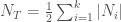$N_T = \frac{1}{2} \sum_{i=1}^k|N_i|$ . This is the figure that is most often reported by the media. As is evident, it is impossible to determine the economic significance of this number without first knowing the structure of the market. That is, we must know how much is owed and to whom. However, after we have this information, we can choose different recovery values and then calculate each party’s exposure. This would enable us to determine how much cash each participant would have to set aside for a default at various recovery values (simply calculate each party’s exposure at the various recovery values).

Let’s consider a concrete example. In the diagram below, an edge coming from a participant represents protection sold by that participant and consequently an incoming edge represents protection bought by that participant. The amounts written beside these edges represent the notional amount of protection bought/sold. The amounts written beside the nodes represent the net notional amounts.

cds-market-diagram

In the example above, D is a dealer and his net notional amount is zero, and therefore his exposure to the risk-event is $0 \cdot M = 0$ . As is evident, we can vary the recovery value to determine what each market participant’s exposure would be in that case. We could then consider other risk-events that occur in conjunction with any given risk-event. For example, we could consider the conjunctive risk-event “ABC defaults and B fails to pay under any CDS” (in which case D’s exposure would not be zero) or any other variation that addresses meaningful concerns. For now, we will focus on our single event risk for explanatory purposes. But even if we restrict ourselves to single event risks, there’s more to a CDS than just default. Collateral will move through the above system dynamically throughout the lives of the contracts. In order to understand how we can analyze the systemic risks posed by the dynamic shifting of collateral, we must first examine what it is that causes collateral to be posted under a CDS.

We’re In The Money

CDS contracts come in and out of the money to a party based on the price of protection. If a party is out of money, the typical market practice is to require that party to post collateral. For example, if I bought protection at a price of 50bp, and suddenly the price jumps to 100bp, I’m in the money and my counterparty is out of the money. Thus, my counterparty will be required to post collateral. We can view the price of protection as providing an implied probability of default. Exactly how this is done is not important. But it should be clear that there is a connection between the cost of protecting debt and the probability of default on that debt (the higher the probability the higher the cost). Thus, as the implied probability of default changes over the life of the agreement, collateral will change hands.

Collateral Flow Analysis

In the previous sections, we assumed that the risk-event was certain to occur and then calculated the exposures based on an assumed recovery value. So, in effect, we were asking “what happens when parties settle their contracts at a given recovery value?” But what if we want to consider what happens before any default actually occurs? That is, what if we want to consider “what happens if the probability of default is $p$ ?” Because collateral will be posted as the price of protection changes over the life of the agreement and the price of protection provides an implied probability of default, it follows that the answer to this question should have something to do with the flow of collateral.

Continuing with the ABC bond example above, we can examine how collateral will move through the system by asking two questions: (i) what is the implied probability of the risk-event (ABC’s default) occurring and (ii) what is the expected value of the risk-magnitude (the basis upon which collateral payments are made). As discussed above, the implied probability of default will change over the life of the agreement, which will in turn affect the flow of collateral in the system. Since our goal in this section is to test the system’s behavior at different implied probabilities of default, the expected value of our risk-magnitude should be a function of an assumed implied probability of default. So, we define the expected value of our risk-magnitude as $M_e = p^* \cdot M$ where $p^*$ is our assumed implied probability of default and $M$ is defined as it is above. It follows that this analysis will break CDS contracts into categories according to the price at which they were entered into. That is, you can’t ask how much something changed without first knowing what it was to begin with.

Assume that $P_i$ entered into CDS contracts at $m_i$ different prices. For example, he entered into four contracts at 20 bp and eight contracts at 50bp, and no others. In this case, $m_i = 2$ . For each $P_i$ , assign an arbitrary ordering, $(c_{i,1}, ... , c_{i,m_i})$ , to the sets of contracts that were entered into at different prices by $P_i$ . In the example where $m_i = 2$ , we could let $c_{i,1}$ be the set of eight contracts entered into at 50bp and let $c_{i,2}$ be the set of four contracts entered into at 20 bp. Each of these sets will have a net notional amount and an implied probability of default (since each is categorized by price). Define $n_{i,j}$ as the net notional amount of the contracts in $c_{i,j}$ and $p_{i,j}$ as the implied probability of default of the contracts in $c_{i,j}$ for each $1 \leq j \leq m_i$ . 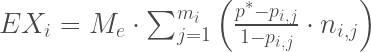We define the expected exposure of $P_i$ as:

$EX_i = M_e \cdot \sum_{j = 1}^{m_i}\left(\frac{p^* - p_{i,j}}{1 - p_{i,j}} \cdot n_{i,j}\right)$ .

Note that when $p^* = 1$ ,

$EX_i = M \cdot \sum_{j = 1}^{m_i}\left(\frac{1 - p_{i,j}}{1 - p_{i,j}} \cdot n_{i,j}\right) = M \cdot N_i$ .

That is, this is a generalized version of the settlement analysis above, and when we assume that default is certain, collateral flow analysis reduces to settlement flow analysis.

So What Does That Awful Formula Tell Us?

A participant’s expected exposure is a reasonable estimate for the amount of collateral that will be posted or received by that participant at an assumed implied probability of default. The exact amount of collateral that will be posted or received under any contract will be determined by the terms of that contract. As a result, our model is approximate and not exact. However, the direction that collateral moves in our model is exact. That is, if a party’s expected exposure is negative, it will not receive collateral, and if it is positive, it will not post collateral. It also shows that even if a party is completely hedged in the event of a default, it is possible that it is not completely hedged to posting collateral. That is, even if it bought and sold the same notional amount of protection, it could have done so at different prices.