Symmetry of Gravity, Dark Matter, and Dark Energy

January 23, 2026January 23, 2026 / erdosfan / Leave a comment

Introduction

I’ve written about the symmetry of gravity in the past, but at the time, I had a much more convoluted theory of physics. I now no longer believe in Quantum Mechanics (at all), and no longer believe in time as anything other than a measurement of change, but you can still of course have time dilation even with this limited definition. See, A Computational Model of Physics, where I rewrote all of Relativity and most of known physics using objective time. Now that I’ve gotten this garbage out of my brain, I have a very simple theory of Dark Matter and Dark Energy.

Dark Matter is predicted to exist because cosmological observations deviate from Relativity. Now, real mathematicians and scientists have garbage cans, and when observation deviates from predictions produced by a model, we throw the model in the garbage. So the best explanation for Dark Matter, is that it doesn’t exist, and Relativity is wrong. We already know that Relativity is wrong for other reasons, e.g., the existence of the Neutrino, which has mass, yet a velocity of c, which is completely impossible in Relativity. But rather than accept this, ostensible scientists fuss about whether it’s exactly c, or some other handwaving nonsense, in defense of a physically implausible theory of the Universe, where everything depends upon anthropomorphic observers, as if electrons had a brain. So I think the best answer for Dark Matter, is that Relativity is wrong, and we need a new model of physics to explain cosmological observations.

In contrast, I don’t think Dark Energy depends upon Relativity. If however, it does depend upon Relativity, then we should start with the assumption that Dark Energy doesn’t exist, and build a new model of physics that is consistent with cosmological observations, otherwise known as doing science. All of that said, it dawned on me last night, that there might be something to Dark Energy, specifically, if we complete the symmetry of gravity.

Let’s start by completing the symmetry of gravity, which requires positive and negative mass, which we will denote as $m$ and $\bar{m}$ , respectively. Let’s further assume that we are surrounded almost exclusively by positive mass, which again is denoted by $m$ . Let’s assume that positive mass is attracted to positive mass, which would obviously be perfectly consistent with gravity, since we’ve already assumed that almost all matter we are exposed to is positive mass. Further, let’s assume that negative mass is similarly attracted to negative mass, and that masses with opposite signs cause repulsion. That is, given some quantity of positive mass $m$ and negative mass $\bar{m}$ , the two masses will repel each other when sufficiently proximate. This completes the symmetry of gravity, since we now have positive and negative masses, and attractive and repulsive forces.

The obvious question is, where’s all this negative mass, and repulsive force? Well, first let’s consider that the Universe is quite old, and as a result, if we posit such a force has always existed, then this would eventually divide the Universe into at least two regions, one filled with mostly positive mass, and one filled with mostly negative mass. If this process is less than complete, then we should see some inexplicable acceleration due to interactions between positive and negative masses, which is consistent with Dark Energy.

Now, the SLAC 144 Experiment demonstrates that light on light collisions can produce matter-antimatter pairs. Further, we know that matter-antimatter collisions can create light. Let’s assume again that we’re in a positive matter region of the Universe, and as such, if we allow $\gamma$ to represent a photon, we could write that $e^+ + e^- = \gamma$ , to represent a positron and electron colliding to form a photon. Similarly, we could write that $\gamma_1 + \gamma_2 = e^+ + e^-$ to represent a light on light collision producing an electron-positron pair.

With that notation, now let’s posit the negative-mass versions of the electron and positron, which we will denote as $\bar{e}^+$ and $\bar{e}^-$ . The question is, what do we get when we combine the negative-mass versions of an electron and positron? Expressed symbolically, $\bar{e}^+ + \bar{e}^- = X$ , where $X$ is some unknown particle.

If it’s an ordinary photon, then we arguably have a problem, because photon collisions have been shown to produce positive-mass electron positron pairs. That is, under this hypothetical, in the negative-mass regions of the Universe, when you do light on light collisions, you still get positive-mass pairs, which should eventually be kicked out of that region of space. In contrast, in the positive-mass regions of the Universe, when you do light on light collisions, you also get positive-mass pairs, but they stick around because it’s ordinary mass.

We could hypothesize that this is just the way things are, but we get an elegant potential solution to the source of Dark Energy if we instead posit the existence of negative-mass light $\bar{\gamma}$ , as a particle distinct from ordinary light. Specifically, if we further posit that negative-mass light does not interact with positive mass, and that positive-mass light (our ordinary photons) do not interact with negative mass, then that negative mass would not be detectable using ordinary photons. Ironically, this is a kind of “dark” matter, but it’s not the nonsense hypothesized hitherto.

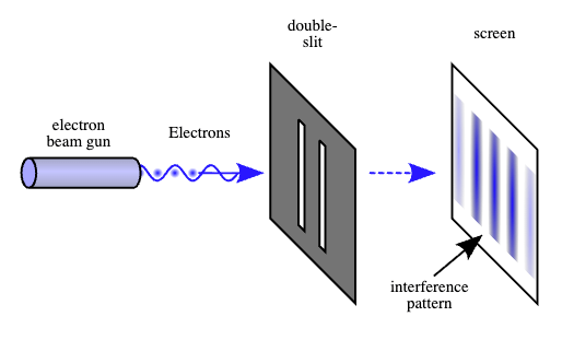
A Fundamental Problem with the Double-Slit Experiment

December 29, 2025December 29, 2025 / erdosfan / Leave a comment

I noticed a while back that the purported Quantum Mechanical explanations for the Double-Slit Experiment, don’t make any sense for a very simple reason: generally, people assume the velocity of light is fixed at c. In contrast, if we assume self-interference for a photon, then the photon must (i) change direction or (ii) change velocity, or both, otherwise, there won’t be any measurable effects of self-interference, barring even more exotic assumptions.

A diagram of the Double-Slit Experiment. Image courtesy of Wikipedia.

We can rule out case (ii), since photons are generally assumed to travel at a constant velocity of c in a vacuum. However, case (i) produces exactly the same problem, since if the photon changes direction due to self-interference, then the arrival time against the screen will imply a velocity of less than c, since by definition, the photon will not have followed a straight path from the gun to the screen. This is the end of the story, and I cannot believe that no one has pointed this out before.

We can instead posit a simple explanation for the purported interference pattern: the photons scatter inside the slit (i.e., bounce around), which from our perspective is flat, but from the perspective of a photon, is instead a tunnel, since the photon (or other elementary particle) is so small. This will produce two distributions of scattering angles (one for each slit), which will overlap at certain places along the screen more than others, producing a distribution of impact points that would otherwise look like a wave interference pattern.

This is much simpler isn’t it, and clearly a better explanation than some exotic nonsense about time and other realities. That’s not how you do science. Now, it could be that there is some experiment that requires such exotic theories, but I don’t know of one, not even the Quantum Eraser Experiment. All of these experiments have simple explanations, and we’ve developed a horrible, unscientific habit, of embracing exotic explanations for basic phenomena, that is at this point suspicious, given the military and economic value of science.

Solution to the Liar’s Paradox

December 19, 2025December 19, 2025 / erdosfan / Leave a comment

I don’t remember the first time I heard about the Liar’s Paradox, but it was definitely in college, because it came up in my computer theory classes in discussions on formal grammars. As such, I’ve been thinking about it on and off, for about 20 years. Wikipedia says that the first correct articulation of the Liar’s Paradox is attributed to a Greek philosopher named Eubulides, who stated it as follows: “A man says that he is lying. Is what he says true or false?” For purposes of this note, I’m going to distill that to the modern formulation of, “This statement is false.”

As an initial matter, we must accept that not all statements are capable of meaningful truth values. For example, “Shoe”. This is just a word, that does not carry any intrinsic truth value, nor is there any meaningful mechanical process that I can apply to the statement to produce a truth value. Contrast this with, “A AND B”, where we know that A = “true” and B = “false”, given the typical boolean “AND” operator. There is in this case a mechanical process that can be applied to the statement, producing the output “false”. Now, all of that said, there is nothing preventing us from concocting a lookup table where, e.g., the statement “Shoe” is assigned the value “true”.

Now consider the distilled Liar’s Paradox again: “This statement is false”. There is no general, mechanical process that will evaluate such a statement. However, it is plainly capable of producing a truth value, since it simply asserts one for itself, much like a lookup table. Typically, this is introduced as producing a paradox, because if we assume the truth value is false, then the truth value of false is consistent with the truth value asserted in the statement. Generally speaking, when assertion and observation are consistent, we say the assertion is true, and this is an instance of that. As such, the statement is true, despite the fact that the statement itself asserts that it is false. Hence, the famous paradox.

Now instead approach the problem from the perspective of solving for the truth value, rather than asserting the truth value. This would look something like, “This statement is A”, where $A \in \{true, false\}$ . Now we can consider the two possible values of $A$ . If $A = true$ , then the statement asserts a truth value that is consistent with the assumed truth value, and there’s nothing wrong with that. If instead $A = false$ , then we have a contradiction, as noted above. Typically, when engaging in mathematics, contradictions are used to rule out possibilities. Applying that principle in this case yields the result that $A = true$ , which resolves the paradox.

In summary, not all statements are capable of mechanical evaluation, and only a subset of those mechanically evaluable statements resolve to true or false. This however does not prevent us from simply assigning a truth value to a statement, whether by a lookup table, or within the statement itself. However, if we do so, we can nonetheless apply basic principles of logic and mathematics, and if we adhere to them, we can exclude certain purported truth values that are the result of mere assertion. In this case, such a process implies that a statement that asserts its own truth value, is always true.

Compton Scattering

December 16, 2025December 16, 2025 / erdosfan / Leave a comment

Introduction

My work in physics relies heavily on the Compton Wavelength, which as far as I know, was introduced solely to explain Compton Scattering. Wikipedia introduces the Compton Wavelength as a “Quantum Mechanical” property of particles, which is nonsense. Compton Scattering instead plainly demonstrates the particle nature of both light and electrons, since the related experiment literally pings an electron with an X-ray, causing both particles to scatter, just like billiard balls. I obviously have all kinds of issues with Quantum Mechanics, which I no longer think is physically real, but that’s not the point of this note.

Instead, the point of the note, is the implications of a more generalized form of the equation that governs Compton Scattering. Specifically, Arthur Compton proposed the following formula to describe the phenomena he observed when causing X-rays (i.e., photons) to collide with electrons.

$\lambda' - \lambda = \frac{h}{m_ec} (1 - \cos(\theta))$ ,

where $\lambda'$ is the wavelength of the photon after scattering, $\lambda$ is the wavelength of the photon before scattering, $h$ is Planck’s constant, $m_e$ is the mass of an electron, $c$ is the velocity of light, and $\theta$ is the scattering angle of the photon. Note that $\frac{h}{m_ec}$ , which is the Compton Wavelength, is a constant in this case, but we will treat it as a variable below.

For intuition, if the inbound photon literally bounces straight back at $\theta = 180\textdegree$ , then $(1 - \cos(\theta))$ evaluates to $2$ , maximizing the function at $\lambda' - \lambda = 2 \frac{h}{m_ec}$ . Note that $\lambda' - \lambda$ is the difference between the wavelength of the photon, before and after collision, and so in the case of a $180\textdegree$ bounce back, the photon loses the most energy possible (i.e., the wavelength becomes maximally longer after collision, decreasing energy, see Planck’s equation for more). In contrast, if the photon scatters in a straight line, effectively passing through the electron at an angle of $\theta = 0\textdegree$ , then $(1 - \cos(\theta)) = 0$ , implying that $\lambda' - \lambda = 0$ . That is, the photon loses no energy at all in this case. This all makes intuitive sense, in that in the former case, the photon presumably interacts to the maximum possible extent with the electron, losing the maximum energy possible, causing it to recoil at a $180\textdegree$ angle, like a ball thrown straight at a wall. In contrast, if the photon effectively misses the electron, then it loses no energy at all, and simply continues onward in a straight line (i.e., a $0\textdegree$ angle).

All of this makes sense, and as you can see, it has nothing to do with Quantum Mechanics, which again, I think is basically fake at this point.

Treating Mass as a Variable

In the previous section, we treated the Compton Wavelength $\frac{h}{m_ec}$ as a constant, since we were concerned only with photons colliding with electrons. But we can consider the equation as a specific instance of a more general equation, that is a function of some variable mass $m$ . Now this obviously has some unstated practical limits, since you probably won’t get the same results bouncing a photon off of a macroscopic object, but we can consider e.g., heavier leptons like the Tau particle. This allows us to meaningfully question the equation, and if it holds generally as a function of mass, it could provide an insight into why this specific equation works. Most importantly for me, I have an explanation, that is consistent with the notion of a “horizontal particle” that I developed in my paper, A Computational Model of Time Dilation [1].

So let’s assume that the more general following form of equation holds as a function of mass:

$\Delta = \lambda' - \lambda = \frac{h}{mc} (1 - \cos(\theta))$ .

Clearly, as we increase the mass $m$ , we will decrease $\Delta$ for any value of $\theta$ . So let’s fix $\theta = 180\textdegree$ to simplify matters, implying that the photon bounces right back to its source.

The fundamental question is, why would the photon lose less energy, as a function of the mass with which it interacts? I think I have an explanation, that actually translates well macroscopically. Imagine a wall of a fixed size, reasonably large enough so that it can be reliably struck by a ball traveling towards it. Let’s posit a mass so low (again, nonetheless of a fixed size) that the impact of the ball actually causes the wall to be displaced. If the wall rotates somewhat like a pinwheel, then it could strike the ball multiple times, and each interaction could independently reduce the energy of the ball.

This example clearly does not work for point particles, though it could work for waves, and it certainly does work for horizontal particles, for which the energy or mass (depending upon whether it is a photon or a massive particle) is spread about a line. You can visualize this as a set of sequential “beads” of energy / mass. This would give massive particles a literal wavelength, and cause a massive particle to occupy a volume over time when randomly rotating, increasing the probability of multiple interactions. For intuition, imagine randomly rotating a string of beads in 3-space.

Astonishingly, I show in [1], that the resultant wavelength of a horizontal massive particle is actually the Compton Wavelength. I also show that this concept implies the correct equations for time-dilation, momentum, electrostatic forces, magnetic forces, inertia, centrifugal forces, and more generally, present a totally unified theory of physics, in a much larger paper that includes [1], entitled A Combinatorial Model of Physics [2].

Returning to the problem at hand, the more massive a particle is, the more inertia it has, and so the rotational and more general displacement of the particle due to collision with the photon will be lower as a function of the particle’s mass. Further, assuming momentum is conserved, if the photon rotates (which Compton Scattering demonstrates as a clear possibility), regardless of whether it loses energy, that change in momentum must be offset by the particle with which it collides. The larger the mass of the particle, the less that particle will have to rotate in order to offset the photon’s change in momentum, again decreasing the overall displacement of that particle, in turn decreasing the probability of more than one interaction, assuming the particle is either a wave or a horizontal particle.

Conclusion

Though I obviously have rather aggressive views on the topic, if we accept that Compton’s Scattering equation holds generally (and I’m not sure it does), then we have a perfectly fine, mechanical explanation for it, if we assume elementary particles are waves or horizontal particles. So assuming all of this holds up, point particles don’t really work, which I think is obvious from the fact that light has a wavelength in the first instance, and is therefore not a point in space, and must at least be a line.

Meaningful Mathematical Relationships

November 9, 2025November 10, 2025 / erdosfan / Leave a comment

I started thinking about correlation again, and it dawned on me, that when we do math and science, we’re looking for computable relationships between sets of numbers. The most basic example is a function that describes the behavior of a system. Ideally, we have exact descriptions, but we often settle for probabilistic descriptions, or descriptions that are exact within some tolerance. I’d say that the search for computable relationships between sets of numbers is in fact science. But when you consider the full set of relationships between two sets of numbers, the set we’re interested in is therefore minuscule in terms of its density. In the extreme case, the set of computable functions has a density of zero compared to the set of non-computable functions. Yet, science and mathematics have come to the point where we can describe the behaviors of far away worlds, and nanoscopic terrestrial systems.

Therefore, it’s tempting to think that the computable is everything, and the balance of relationships are nonsense. For physical intuition, consider a Picasso painting represented as an RGB image, and compare that to the full set of random RGB images of the same size. What’s strange, is that the set in question will contain other known masterpieces, and new unknown masterpieces, if the image is large enough and the pixel size is small enough. And while I haven’t done the math, I’d wager the density of masterpieces is quite small, otherwise we’d all be famous painters, and since we’re not, I don’t think you can gamble your way into a masterpiece.

Similarly, if I have two sets of random numbers, and I simply connect them with strings, you’d probably think I’m a lunatic, though I’ve just defined a function. Whereas if I point out that I can inject the set of integers into the set of even integers, you’d swear I’m a genius. This might seem like unscientific thinking, but it isn’t. It’s arguably all the same, in that humans have a clear preference for computability, and that translates into a preference for symmetry over asymmetry. Personally, I listen to a lot of strange, highly random music, and enjoy Gregory Chaitin’s work as well, but in all seriousness, are we missing valuable information in the form of more complex functions, and perhaps tragically in the form of non-computable functions, assuming no non-computable machine exists?

Halting Processes and Proofs

November 2, 2025November 3, 2025 / erdosfan / Leave a comment

I was again reading my absolute favorite book on mathematics, Mathematical Problems and Proofs [1] (no, I am not paid for this endorsement, it really is that great), and on page 11 of the text, Example 1.20 gives Euclid’s Theorem on Prime Numbers, demonstrating that the set of prime numbers must be infinite. I immediately recalled that all natural numbers are either prime, or the product of primes, known as the Fundamental Theorem of Arithmetic. This is a different result, the proof of which is not presented in [1] (at least I didn’t see it).

I checked Google, and there’s a straightforward proof using induction, but it lacks intuitive appeal. As such, I spent a few minutes this morning thinking about it, and I realized you can construct an intuitive proof. I haven’t seen this proof elsewhere, though it could be a known result. Even if it is known, what’s interesting is the structure of the proof, which is you can show that it must be the case that the algorithm upon which the proof relies, will eventually halt. This is pretty interesting, and maybe it’s a new form of proof. At a minimum, we have an intuitive proof of the Fundamental Theorem of Arithmetic that does not rely on induction.

The Proof

Assume you have a natural number $n \in \mathbb{N}$ . If $n$ is prime, then we’re done. So assume that $n$ is not prime. As such, it must be the case that $n = a_1b_1$ , for $a_1,b_1 \in \mathbb{N}$ , and therefore, $a_1 = \frac{n}{b_1} \in \mathbb{N}$ . The intermediate result will be to show that all numbers are either prime, or have at least one prime factor, which we will then use to prove the Fundamental Theorem of Arithmetic. As such, if $a_1$ is prime, then we’re done. Therefore, assume $a_1$ is not prime, and as such, $a_2 = \frac{a_1}{b_2}$ , for $a_2,b_2 \in \mathbb{N}$ . We can of course continue to apply this process for increasing values of $i \in \mathbb{N}$ , generating decreasing values of $a_i$ . However, there are only finitely many numbers less than $n$ , and as such, this process must eventually terminate, producing a prime number $a_m = \frac{a_{m-1}}{b_m}$ . Note that $a_m = \frac{n}{b_1 \cdots b_m}$ , and as such, $n = a_m (b_1 \cdots b_m)$ . Therefore, all natural numbers have at least one prime factor.

Now let’s express $n$ as the product of this prime number $p_1 = a_m$ , and the remaining factors, $f_1 = b_1 \cdots b_m$ , i.e., $n = p_1f_1$ . Note that $f_1$ cannot be prime, so we can therefore run the algorithm above on $f_1$ , which will produce another prime number factor $p_2$ , and another remaining factor $f_2$ , such that $n = p_1p_2f_2$ . Note that it must be the case that $f_2 < f_1$ , and in general, $f_{i+1} < f_i$ , and therefore it requires fewer steps to calculate each successive prime factor. Because the number of steps is always a natural number, this process must terminate. Therefore, $n$ will eventually be expressed as the product of a finite number of primes.

Higher Order Relations

June 15, 2025June 15, 2025 / erdosfan / Leave a comment

I was reading my favorite book on mathematics, Mathematical Problems and Proofs, in particular, a section on basic Set Theory. The book discusses the transitive relation, where if A is related to B, and B is related to C, then A is related to C. In this case, A, B, and C are abstract mathematical objects, but you can assign practical meaning by e.g., making them all integers, and considering ordinal relationships between them, where e.g., A is greater than B, B is greater than C, and therefore, A is greater than C. Note that this example of ordinal relationships has a “therefore” clause, but relations are abstract statements of fact, not consequences of logic. That is, we simply posit relations between objects, whereas I’ve phrased the concrete example in terms of a logical conclusion, which is very different. That is, this example is consistent with the stated set of relations among A, B, and C, which are simply posited to exist, whereas the integers have properties that imply that A is greater than C as a matter of logic.

With that introduction, it dawned on me that we can consider higher order sets of relations that probably don’t have names like “transitive”. One obvious such set of relations is as follows, where A is related B, B is related to C, C is related to D, and A is related to D. All I did was add an extra object D, and extend the relations analogously. Specifically, we can express this as a graph, where A through D are connected by a path, and A is connected directly to D by an extra edge, creating what would be a circuit in an undirected graph. Though note that even if A is related to B, this does not imply that B is related to A, and as such, any graph expressing relations is directed. This is probably known, given how simple it is, and I’m certain through my own studies that people express relations using graphs.

The interesting bit is the possibility of using machines to discover meaningful higher order relations that e.g., require at least four or more objects. Because it’s at least possible for these relations to arise over any number of objects, we can’t give them all special names in a human language like “transitive”, but a machine can. The point being that, most of mathematics is probably accessible only to machines or other sentient beings capable of handling that much information, which plainly do not inhabit this planet in any appreciable number.

Thought on the Double Slit Experiment

October 29, 2024October 29, 2024 / erdosfan / Leave a comment

I realized the other day that the equations I present in Section 3.3 of my paper, A Computational Model of Time-Dilation, might imply that wave behavior will occur with a single particle. I need to go through the math, but the basic idea is that each quantized chunk of mass energy in an elementary particle is actually independent, and has its own kinetic energy. This would allow a single elementary particle to effectively sublimate, behaving like a wave. The point of the section is that on average, it should still behave like a single particle, but I completely ignored the possibility that it doesn’t, at least at times, because I wanted single particle behavior, for other sections of the paper. I was reminded of this, because I saw an experiment, where a single neutron plainly travels two independent paths. If the math works out, we could completely ditch superposition, since there’s no magic to it, the particle actually moves like a wave, but generally behaves like a single particle. That said, I think we’re stuck with entanglement, which seams real, and I still don’t understand how it works, but nothing about entanglement contradicts my model of physics.

Spatial Uncertainty and Order

September 28, 2024September 28, 2024 / erdosfan / Leave a comment

I presented a measure of spatial uncertainty in my paper, Sorting, Information, and Recursion [1], specifically, equation (1). I proved a theorem in [1] that equation (1) is maximized when all of its arguments are equal. See, Theorem 3.2 of [1]. This is really interesting, because the same is true of the Shannon Entropy, which is maximized when all probabilities are equal. They are not the same equation, but they’re similar, and both are rooted in the logarithm. However, my equation takes real number lengths or vectors as inputs, whereas Shannon’s equations takes probabilities as inputs.

I just realized, that Theorem 3.2 in [1], implies the astonishing result, that the order of a set of observations, impacts the uncertainty associated with those observations. That is, we’re used to taking a set of observations, and ignoring the ordinal aspect of the data, unless it’s explicitly a time series. Instead, Theorem 3.2 implies that the order in which the data was generated is always relevant in terms of the uncertainty associated with the data.

This sounds crazy, but I’ve already shown empirically, that these types of results in information theory work out in the real world. See, Information, Knowledge, and Uncertainty [2]. The results in [2], allow us to take a set of classification predictions, and assign a confidence value to them, that are empirically correct, in the sense that accuracy increases as a function of confidence. The extension here, is that spatial uncertainty is also governed by an entropy-type equation, specially equation (1), which is order dependent. We could test this empirically, by simply measuring whether or not prediction error, is actually impacted by order, in an amount greater than chance. That is, we filter predictions, as a function of spatial uncertainty, and test whether or not prediction accuracy improves as we decrease uncertainty.

Perhaps most interesting, because equation (1) is order dependent, if we have an observed uncertainty for a dataset (e.g., implied from prediction error), and we for whatever reason do not know the order in which the observations were made, we can then set equation (1) equal to that observed uncertainty, and solve for potential orderings that produce values approximately equal to that observed uncertainty. This would allow us to take a set of observations, for which the order is unknown, and limit the space of possible orderings, given a known uncertainty, which can again be implied from known error. This could allow for implications regarding order that exceed a given sample rate. That is, if our sample rate is slower than the movement of the system we’re observing, we might be able to restrict the set of possible states of the system using equation (1), thereby effectively improving our sample rate in that regard. Said otherwise, equation (1) could allow us to know about the behavior of a system between the moments we’re able to observe it. Given that humanity already has sensors and cameras with very high sample rates, this could push things even further, giving us visibility into previously inaccessible fractions of time, perhaps illuminating the fundamental unit of time.

Knowledge and Utility

July 6, 2024July 6, 2024 / erdosfan / Leave a comment

I wrote a paper a while back called “Information, Knowledge, and Uncertainty” [1], that presents a mathematical theory of epistemology. I go on to apply it, showing that it can be used in machine learning to drastically improve the accuracy of predictions, using a measure of confidence that follows from the definitions in [1]. In some other research note that I don’t remember the name of, I pointed out that we can also think about a different kind of information that is conveyed through a proof. Specifically, that longer proofs correspond to more computational work, i.e., the work required to prove the theorem, which will have some number of deductive steps. Simply count the steps, the more steps there are, the more work required to prove the result. Now of course, you could have a “bad” and pointlessly long proof for a theorem. Simply posit the existence of a shortest proof, as an analog to the Kolmogorov Complexity. The number of steps in the shortest proof for a theorem is the depth of the theorem.

What caught my attention this morning is the potential connection between utility and the depth of a theorem. For example, the Pythagorean Theorem has very short proofs, and as a result, the shortest proof will necessarily also be short. Despite this, the Pythagorean Theorem is remarkably useful, and has undoubtedly been used relentlessly in architecture, art, and probably plenty of other areas of application. Now you could argue that there is no connection between depth and utility, but perhaps there is. And the reason I think there might be, is because I show that in [1], the more Knowledge you have in a dataset, the more accurate the predictions are, implying utility is a function of Knowledge, which has units of bits.

You can view the number of steps in a proof as computational work, which has units of changes in bits, which is different than bits, but plainly a form information. So the question becomes, is this something universal, in that when information is appropriately measured, that utility becomes a function of information? If this is true, then results like the Graph Minor Theorem and the Four Color Theorem could have profound utility, since these theorems are monstrously deep results. If you’re a cartographer or someone that designs flags, then the Four Color Theorem is already useful, but jokes aside, the point is, at least the potential, for profound utilization of what are currently only theoretical results.

As a self-congratulatory example, I proved a mathematical equivalence between sorting a list of real numbers and the Nearest Neighbor method [2]. The proof is about one page, and I don’t think you can get much shorter than what’s there. But, the point is, in the context of this note, that the utility is unreal, in that machine learning is reduced to sorting a list of numbers (there’s another paper that proves Nearest Neighbor can produce perfect accuracy).

I went on to demonstrate empirically that the necessarily true mathematical results work, in the “Massive” edition of my AutoML software BlackTree AutoML. The results are literally a joke, with my software comically outperforming Neural Networks by an insurmountable margin, with Neural Networks taking over an hour to solve problems solved in less than one second (on a consumer device) using BlackTree, with basically the same accuracy in general. Obviously, this is going to have a big impact on the world, but the real point is, what do the applications of something like the Graph Minor Theorem even look like? I have no idea. There’s another theorem in [2] regarding the maximization of some entropy-like function over vectors, and I have no idea what it means, but it’s true. I’ve dabbled with its applications, and it looks like some kind of thermodynamics thing, but I don’t know, and this is disturbing. Because again, if true, it implies that the bulk of human accomplishment has yet to occur, and it might not ever occur because our leaders are a bunch of maggots, but, if we survive, then I think the vast majority of what’s possible is yet to come.

All of that said, I’m certainly not the first person to notice that mathematics often runs ahead of e.g., physics, but I’m pretty sure I’m the first person to notice the connection (if it exists) between information and utility, at least in a somewhat formal manner. If this is real, then humanity has only scratched the surface of the applications of mathematics to reality itself, plainly beyond physics.

Information Overload

philosophy