I was looking at pictures of Frank Sinatra’s home in Palm Springs, and I noticed that the kitchen looked very similar to a kitchen that I described in a book I wrote, VeGa. You can just take my word for it since it’s a long book, but the similarities are a bit tough to accept as mere coincidence. Now, it’s entirely possible I previously saw pictures of Sinatra’s home, since I’m a huge fan and have been for my entire adult life, but it doesn’t matter to the conclusion that followed, which is that art in particular and aesthetics generally, create an opportunity for information about a person’s genome to be expressed, and therefore, facilitate mating decisions.
I’ve seen some evidence that preferences are genetic, and this should surprise no one, since people clearly take aesthetic preferences seriously, often motivating people to work harder, just so they can live in a particular home, and wear particular clothes. The more formal conclusion I reached this morning is not on the empirical side, it is instead a theoretical observation, that the expression of preferences creates a language in which information about genomes can be conveyed. There is still of course the empirical question of whether or not this is actually happening, but as we’ll see, the opportunity to convey an enormous amount of information using preferences certainly exists.
Let’s begin by formalizing and limiting preferences as expressed with respect to a particular artifact (e.g., a piece of music, a painting, a pair of pants, etc.), as follows: I hate it, I don’t like it, it’s OK, I like it, and I love it. This creates an ordinal scale of 5 possibilities, ranging from hate to indifference to love, that we’ll use to express preferences. In reality, people have written entire books about single paintings, so the real world range of expression, is much wider, but as we’ll see, it doesn’t matter, you already have an incredibly expressive language using just these five possibilities.
Specifically, for any artifacts, there will be possible rankings. As a consequence, two people discussing, e.g., just 10 works of art, creates 9,765,625 possible rankings, and again, all they have to say is, I hate it, I don’t like it, it’s OK, I like it, or I love it, 10 times, and they’ll convey about 23 binary bits of information, which is genetic bases worth of information. As you can see, increasing the number of possible rankings simply increases the base of the exponent, whereas the exponent dominates the counting function.
Common sense says that people will primarily respond to appearance, smell, taste, and other visceral information when selecting mates, but there are still at least two potentially important roles that art and aesthetics could facilitate in mating decisions, and thereby explain its otherwise anomalous importance to humanity: (1) filtering large crowds of individuals on the basis of shared preferences and (2) marginal distinctions within homogenous populations.
Understanding point (1) is straightforward, if you e.g., put together an event that centers around aesthetic artifacts (e.g., a concert, a gallery exhibition, etc.), then generally speaking, people will attend that event only if they’re sufficiently interested in the full set of artifacts, and the particular combination of artifacts in question. That is, even if you like both Keith Haring and Caravaggio, it’s a bit weird to combine both in a single exhibit.
Therefore, we can express the same ordinal rankings over combinations of artifacts, and that drastically increases the amount of information conveyed. Specifically, given artifacts, there are possible combinations of artifacts (i.e., the cardinality of the set of all subsets of artifacts), each of which is capable of an ordinal ranking, and therefore, we have, for any artifacts, possible rankings over the set of all subsets of those artifacts. If we set as we did above, i.e., considering just 10 artifacts, we find that , which is approximately 1187 genetic bases worth of information, or approximately 7.0% of an entire human mtDNA genome. Now we’re talking about a significant amount of information, that can realistically be conveyed, since , and most people should be able to meaningfully consider around 1000 collections of artifacts, at least over a significant period of time. Just imagine selecting an outfit to wear to a particular gallery exhibition, this is exactly the kind of combination of preferences that we’re considering, which quickly start to cover large numbers of possible combinations. In fact, even having strong preferences of this sort could demonstrate genetic fitness, in addition to conveying genetic information. The net point being, because it’s possible, and it’s obviously something many people take very seriously, it should have some biological function, and I think it’s the obvious: you’re conveying information about your genome through your preferences.
Point (2) is not hard to understand given the above, which is that in a genetically and morphologically homogenous society (i.e., everyone is genetically and physically very similar), marginal differences in genomes could be important, in particular because you have a high risk of incest. It’s not clear to me that there’s any real evidence of heightened selection for aesthetics in homogenous societies, but the discussions above suggest it should happen, because you can convey marginal differences in genetics through your preferences, allowing people to maximize genetic diversity in an otherwise homogenous population.
I was stuck at Neanderthal Genome 8 in my dataset, which you can find here on the NIH website. I simply could not construct a reasonable history for it using the rest of the Neanderthal genomes. However, just like the other presumably misclassified Neanderthal genomes in my dataset, the provenance file (i.e., the previous link) for Neanderthal Genome 8 also contains a qualified entry in that the “isolate” field is set to “Denisova 15”, suggesting again, that this is actually a Denisovan genome, that is somehow associated with Neanderthals. To test this hypothesis, I compared Neanderthal Genome 8 to all other genomes in my dataset to kick the tires from scratch, and I noticed that Neanderthal Genome 8 is a 98.50% match to a modern African genome from Cameroon. That same Cameroon genome, also tests as Denisovan, specifically, it is a 51.09% match to this Denisovan genome. The logical conclusion, is that Neanderthal Genome 8 was similarly misclassified, and is instead yet another Denisovan genome of African origin.
I now have very little doubt about the Out of Africa hypothesis, and specifically, I think the modern day people of Cameroon are related to the first humans, since every test I’ve come up with points to them as the ancestor of all the archaic genomes in the dataset. Since the modern day Cameroon people test as the ancestors of the archaic genomes, they are presumably even more archaic, but somehow still alive. You can read more about this here. I should be done with the complete history of the Neanderthal and Denisovan lines shortly, it’s just a lot of information and much more complicated than Heidelbergensis, which was astonishingly simple and obvious.
I’m building up to a formal paper on human history that uses Machine Learning applied to mtDNA. You can find an informal but fairly rigorous summary that I wrote here [1], that includes the dataset in question and the code. In this note, I’m going to treat the topic at the individual genome level, whereas in [1], I generally applied algorithms to entire populations at a time (i.e., multiple genomes of the same ethnicity), and looked at genetic similarities across entire populations. The goal here is to tell the story of the Heidelbergensis maternal line, which is the largest maternal line in the dataset, accounting for 414 of the 644 genomes in the dataset (i.e., 62.35%). Specifically, 414 genomes are at least a 90% match to either Heidelbergensis itself, or one of the related genomes we’ll discuss below.
The Dataset
The dataset consists of 644 whole mtDNA genomes taken from the NIH database. There are therefore 644 rows, and columns, each column representing a base of the genome stored in that row (i.e., each column entry is one of the bases A, C, G, or T, though there are some missing bases, represented by 0’s). Said otherwise, each genome contains bases, and each row of the dataset contains a full mtDNA genome.
I’ve diligenced the genome provenance files (see, e.g., this Norwegian genome’s provenance file) to ensure the ethnicity of the individual in question is, e.g., a person that is ethnically Norwegian, as opposed to a resident of Norway. The dataset consists of 75 classes of genomes, which are, generally speaking, ethnicities, and column N+1 contains an integer classifier for each genome, representing the ethnicity of the genome (e.g., Norway is represented by the classifier 7). The dataset also contains 19 archaic genomes, that similarly have unique classifiers, that are treated as ethnicities as a practical matter. For example, there are 8 Neanderthal genomes, each of which have a classifier of 32, and are for all statistical tests treated as a single ethnicity, though as I noted previously, Neanderthals are decidedly heterogenous. So big picture, we have 644 full mtDNA genomes, each stored as a row in a matrix (i.e., the dataset), where each of the first columns contains a base of the applicable genome, and an integer classifier in column N+1, that tells you what ethnicity the genome belongs to.
Heidelbergensis and mtDNA
Heidelbergensis is an archaic human that lived (according to Brittanica) approximately 600,000 to 200,000 years ago. When I first started doing research into mtDNA, I immediately noticed that a lot of modern mtDNA genomes were a 95% or more match to Heidelbergensis. I thought at first I was doing something wrong, though I recently proved (both mathematically and empirically) that this is definitely not the case, and in fact, there’s only one way to compare whole mtDNA genomes. You can read the previous note linked to for details, but the short story is, mtDNA is generally inherited directly from your mother (i.e., there’s no paternal DNA at all in mtDNA), with no mutations, though mutations can occur over long periods of time (i.e., thousands of years, or sometimes more).
As a result, any method you use to compare an entire mtDNA genome must be able to produce nearly perfect matches, since a large enough dataset should contain a basically perfect match for a significant number of genomes, given mtDNA’s extremely slow rate of mutation. Said otherwise, if you have a large number of whole mtDNA genomes, there should be nearly perfect matches for a lot of the genomes in the dataset, since mtDNA mutates extremely slowly. There are of course exceptions, especially when you’re working with archaic genomes that might not have survived to the present, but the gist is, mtDNA mutates so slowly, someone should have basically the same mtDNA as you. Empirically, there’s exactly one method of whole-genome comparison that accomplishes this, which is explained in the previous link and contains the applicable code to test the hypothesis.
Just in case it’s not clear, whole-genome comparison means you take two entire genomes, and compare them side-by-side, rather than looking for individual sequential segments like genes, which until recently, was the more popular approach. If you’re curious, I’ve demonstrated that whole-genome comparison, and random base selection, are categorically superior to relying on sequential bases (e.g., genes) for imputation, at least as applied to mtDNA. See, A New Model of Computational Genomics [2]. We will also discuss using genome segments in the final section below.
A Heidelbergensis skull, image courtesy of Britannica.
Whole-Genome Comparison
The method of comparison that follows from this observation is straight forward, you simply count the number of matching bases between two genomes. So for example, if we’re given genome and , the number of matching bases is simply 2. Because mtDNA is circular, it’s not clear where to start the comparison. For example, we could start reading genome at the first , rather than the first base . However, the previous link demonstrates that there’s exactly one whole-genomealignment (otherwise known as a global alignment), or starting index for mtDNA, the rest of them are simply not credible for the reasons discussed above.
This makes whole-genome comparison super easy, and incredibly fast, and in fact, my software can compare a given genome to all 644 genomes in the dataset in just 0.02 seconds, running on an Apple M2 Pro, producing a ton of statistics for the input genome, not just the number of matching bases. Sure, it’s a great machine, but it’s not a super computer, which means now everyone can do real genetic analysis on consumer devices. Once popularized, these methods will probably make short work of the complete history of mankind, and possibly the entire history of life itself, since mtDNA is not unique to humans. Further, these methods and their results are rock solid, empirical evidence for the Theory of Evolution, which as you’ll see below, is not subject to serious criticism, at least with respect to mtDNA.
Modern Relatives of Heidelbergensis
As noted above, many modern living humans have mtDNA that is a 95% or more match to the single Heidelbergensis genome in the dataset. The genome was found at Sima de Los Huesos, and there is apparently some debate about whether it is actually a Neanderthal, but it is in all cases a very archaic genome from around 500,000 years ago. As such, though I concede this Heidelbergensis genome is a 95.10% match to the third Neanderthal genome in my dataset, which is from around 100,000 years ago, I think it’s best to distinguish between the two, given the huge amount of time between the two genomes, and the fact that they’re not exactly the same genome.
Recall that we are comparing whole-genomes by simply counting the number of matching bases, which we’ll call the match count. We can therefore, set a minimum match count of say , i.e., 90% of the genome, and retrieve all genomes that are at least a 90% match to Heidelbergensis. This produces the chart below, where the height of the bar provides the percentage of genomes in the applicable population that are at least a 90% match to the single Heidelbergensis genome. For example, 100% of the Iberian Romani are at least a 90% match to the Heidelbergensis genome, producing a height of 1.0 in the chart below. The population acronyms can be found at the back of [2], but just to highlight some of the obvious matches, KZ stands for Kazakhstan, IB stands for Iberian Romani, IT stands for Italy, and RU stands for Russia.
A chart showing the percentage of each population that is at least a 90% match to Heidelbergensis.
The plain takeaway is that many modern humans carry mtDNA that is close to Heidelbergensis, peaking at a 96.69% match for a Kazakh individual. As noted above, when working with modern genomes, you’ll often find a basically perfect match that exceeds 99%, but when working with archaic genomes, that’s not always the case, and it makes perfect sense, since so much time has elapsed, that even with the incredibly slow rate of mutation for mtDNA, a few percentage points of mutation drift is to be expected.
The Phoenician People
The Phoenicians were a Mediterranean people that existed from around 2500 BC to 64 AD. Though there could be other example genomes, the Phoenicians are a great case study because they are a partial match to Heidelbergensis, and a partial match to the Pre-Roman Ancient Egyptian genome. You can already appreciate the intuition, that Heidelbergensis evolved into the Phoenicians, and then the Phoenicians evolved further into the Ancient Egyptians.
Now the real story is more complicated, and it doesn’t look like all of this happened in the Mediterranean. Instead, it looks like human life begins in West Africa, migrates to roughly the Mediterranean and Eurasia, migrates further to somewhere around Northern India, and then spreads back to Europe and Africa, and further out into East Asia. You can read [2] for more on this topic, this note will instead be focused on the evolution of the individual genomes, and less so on claims regarding their historical geographies. That is, I’m going to present you with a set of genomes that begin with Heidelbergensis, and end in the Icelandic people, who are almost certainly Vikings, but I’m not going to argue too much about where these mutations happened, outside of a few notes for context, so that it’s not all happening in a void.
Returning to the Phoenicians, we want to show first, that the Phoenicians evolved from Heidelbergensis. All of these steps will involve epistemological reflections, so that we can be comfortable that we’re asserting reasonable claims. That said, as you’ll see, all of these claims are uncertain, and plainly subject to falsification, but that’s science. To begin, note that there are 6 Phoenician genomes in the dataset, and that the first Phoenician genome in the dataset (row 415) is at least a 99.72% match to the other 5 Phoenician genomes. As such, to keep things simple, we will treat this first Phoenician genome as a representative genome for the entire class of Phoenicians. Further, note that the first Phoenician genome is a 41.17% match to Heidelbergensis. If we were comparing two random genomes, then the expected match count is 25% of the genome, since the distribution is given by the Binomial Distribution, with a probability of success of . That is, at each base, we have two random variables, one for each genome, and each of those variables can take on a value of A, C, G, or T. If it’s truly random, then there are possible outcomes, and only 4 of those outcomes correspond to the bases being the same, producing a probability of . Therefore, we can conclude that the match count of 41.17% between Heidelbergensis and the Phoenician genome is probably not the result of chance.
The claim that the two genomes are truly related finds further support in the location of the matching bases, which are concentrated in the first 3,500 bases, which is shown in the chart below. The chart below is produced by taking 500 bases at a time, starting with the first 500 bases of each genome, and counting how many bases within that 500-base segment match between the two genomes. The maximum match count is of course 500 bases, which would produce a height of 1.0, or 100%. This process continues over the entire genomes, producing the chart below. As you can see, the most significant matches are clustered in the first 7 segments, representing the first 3,500 bases of the genomes. The argument is, because there is a significant, contiguous segment within the genomes that are highly similar, we can confidently rule out chance as the driver of the similarity. You can never be totally certain, but since it’s probably not chance that’s driving the similarity, the logical conclusion is that heredity and mutation is what caused the similarity between the two genomes. Now we don’t know the direction of time from this analysis alone (i.e., either genome could have evolved into the other), but because Heidelbergensis is very archaic, the logical conclusion, is that Heidelbergensis mutated, eventually forming the Phoenician maternal line.
A chart showing the percentage of matching bases between the Heidelbergensis and Phoenician genome, broken into 500-base segments.
One important point to note, is that even if a genome evolves, it does not imply that all instances of that genome evolve. For example, as noted above, 100% of the living Iberian Romani people are at least a 90% match to Heidelbergensis, demonstrating that at least some Heidelbergensis genomes did not evolve into the Phoenician line, and instead remained roughly the same over time. As such, we can say confidently that mtDNA is very slow to mutate as a general matter, but the rates of mutation are heterogenous.
Just to close this section with some context for modern humans that carry the Phoenician line, 80% of living Sardinians and 33.33% of living Vedda Aboriginals are at least a 90% match to the Phoenicians. Obviously, it’s a bit shocking that you’d have Phoenician mtDNA in Asia, but if you read [2], you’ll quickly learn that these are global maternal lines that often contain multiple disparate people. Two common sense explanations, (1) the Phoenicians really made it to Asia or (2) there’s a common ancestor for both the Phoenician and Vedda people, presumably somewhere in Asia. Hypothesis (2) finds support in the fact that 10.52% of Mongolians are also at least a 90% match to the Phoenicians. This is a complicated topic, and it’s just for context, the real point of this note is that you can plainly see that Heidelbergensis evolved, which is already interesting and compelling evidence for the Theory of Evolution, and specifically, it evolved into the Phoenician maternal line.
The Ancient Egyptians
Introduction
The Ancient Egyptians were a Mediterranean civilization that lasted from around 3150 BC to 30 BC, until it was ruled by Rome, from around 30 BC to 642 AD. There are two Ancient Egyptian genomes in the dataset, one from approximately 2000 BC, before Roman rule, and another genome from approximately 129 to 385 AD, during Roman rule. This is a huge amount of time, and so it’s not surprising that the demographics changed. But the Ancient Egyptians present a shocking demographic shift, from earlier rulers that were plainly of Asian origin, to rulers that looked, and were known to be, European. For example, see the panel of images below, with Nefertiti (1353 to 1336 BC) on the left, then King Menkaure and his Queen (2550 BC to 2503 BC), and finally Cleopatra (51 to 30 BC) on the right, who is known to be Macedonian.
Queen Nefertiti, image courtesy of Wikipedia.King Menkaure and Queen, image courtesy of Museum of Fine Arts Boston.Queen Cleopatra, image courtesy of Wikipedia.
The hypothesis that the earlier Egyptians were of Asian origin is further supported by the chart below, which shows the distribution of genomes that are at least a 99% match to the Pre-Roman Egyptian genome. The full set of population acronyms are in [2], but for now note that NP stands for Nepal, JP stands for Japan, FN stands for Finland, NO stands for Norway, EG stands for modern day Egypt, DN stands for Denmark, GA stands for Georgia, TH stands for Thailand, FP stands for Philippines, and KR stands for Korea. As you can plainly see, the Pre-Roman Egyptian genome is very common in Northern Europe and East Asia, with very little representation in Africa outside of modern day Egypt, though there is some nuance to this. See [2] for more. The point is, the Pre-Roman Egyptian genome probably comes from Asia, and spread to Northern Europe, North Africa, and East Asia, and as far as I know, this is not exactly accepted history, but it’s clearly the case.
A chart showing the percentage of each population that is at least a 99% match to the Pre-Roman Egyptian genome.
Ancestry from Heidelbergensis and Phoenicia
As noted above, the Pre-Roman Egyptian genome (row 320) is a partial match to the Phoenician genome, with a match count of 88% of the genome. This is obviously very high, so we can be confident that this is not the result of chance, and is instead the result of heredity and mutation. Further, because we have assumed that Heidelbergensis is the ancestor of the Phoenician genome (since it is archaic), it cannot be the case that the Ancient Egyptian genome is also the ancestor of the Phoenician genome. Specifically, because mtDNA is inherited directly from the mother to its offspring, there can be only one ancestral maternal line for a given genome, though there can be intermediate ancestors. For example, genome A mutates into genome B, which in turn mutates into genome C. However, because the Ancient Egyptian genome has a match count of 29.73% to Heidelbergensis, the Ancient Egyptian genome cannot credibly be an intermediate ancestor of the Phoenicians, between Heidelbergensis and the Ancient Egyptians. Therefore, it must be the case, given our assumption that Heidelbergensis is the ancestor of the Phoenicians, that the Pre-Roman Ancient Egyptian genome is the descendant of the Phoenicians.
Historically, this is counterintuitive, because the Ancient Egyptians are more ancient than the Phoenicians, but as noted above, these maternal lines are broader groups, I’m simply labelling them by using the most famous civilizations that have the genomes in question. Further, as noted above, a lot of this evolution probably happened in Asia, not the Mediterranean. So one sensible hypothesis is that Heidelbergensis travelled East, mutated to the Phoenician line somewhere in Asia, and then that Phoenician line mutated further into the Pre-Roman Ancient Egyptian line, again probably somewhere in Asia. This is consistent with the fact that 76.67% of Kazakh genomes, 44.44% of Indian genomes, and 66.67% of Russian genomes are at least a 95% match to Heidelbergensis, making it plain that Heidelbergensis travelled to Eurasia and Asia. In contrast, as noted above, the Pre-Roman Ancient Egyptian line is found generally in Northern Europe, East Asia, and North Africa, consistent with a further migration from Eurasia and Asia, into those regions.
The Roman Era Egyptian Genome
As noted above, the Ancient Egyptians were ruled by Rome from around 30 BC to 642 AD. Though it is reasonable to assume that there were resultant demographic changes, we’re only looking at two genomes from Ancient Egypt, and so the point is not that these two genomes are evidence of that demographic change. The evidence of the demographic changes are above, in the form of archeological evidence of completely different people ruling their civilization. The point of this section is instead that there is a second genome that was found in Egypt, that is dated to around 129 to 385 AD, squarely during Rome’s rule over Egypt, that is related to the other Ancient Egyptian genome discussed above. Specifically, the Roman Era Egyptian genome (row 321) is a 42.20% match to the Pre-Roman Egyptian genome (row 320). Now, that is significantly above chance (i.e., 25%), but we can also perform the same analysis we did above, looking to 500-base segments for confirmation that the match count is not the result of chance, which is shown below. Again, the most similar regions are concentrated in the first seven, 500-base segments, plainly suggesting heredity rather than chance.
Because we have assumed the Phoenician genome is the ancestor of the Pre-Roman Egyptian genome, it cannot be the case that the Roman Era Egyptian genome is the ancestor of the Pre-Roman Egyptian genome. We can further rule out the possibility of an intermediate relationship by noting that the match count between the Roman Era Egyptian genome and the Phoenician genome is 30.50%. Therefore, we have established a credible claim that Heidelbergensis evolved into the Phoenician maternal line, which in turn evolved into the Pre-Roman Egyptian maternal line, and then further into the Roman Era Egyptian maternal line.
Iceland and the Vikings
The dataset contains a single Icelandic genome, though it was collected from a person in Canada. So it’s fair to express some skepticism, as people can deliberately deceive researchers, though I’m not sure why you would. But that said, let’s kick the tires, and see what populations are at least a 99% match to this purportedly Icelandic genome, which is shown in the chart below. Because these genomes are members of large global groups, we need to be careful in this type of analysis, and accept uncertainty. But you can plainly see in the chart below, that the genome in question is a pronounced match to Sweden (SW) and Norway (NO). Further, the Icelandic genome is a 99.77% match to the single Dublin genome (DB), and Dublin was a Viking colony. Now all of this is subject to falsification and uncertainty, but I think we can be reasonably confident, that the person in question really is of Icelandic ancestry.
A chart showing the percentage of each population that is at least a 99% match to the Icelandic genome.
With that, we can turn to heredity, in particular noting that the Roman Era Egyptian genome is an 87.79% match to the Icelandic genome. Though that is an extremely high match count, that cannot credibly be the result of chance, we can also examine the structure of the matching segments, just as we did above, since we have some doubt regarding the provenance, given that the individual lived in Canada. This is shown below, and as you can see, it is plainly not the result of chance, since the vast majority of matching segments are from and including segment 7 onward. Because we have assumed that the Pre-Roman Egyptian genome is the ancestor of the Roman Era Egyptian genome, it cannot be the case that the Icelandic genome is the ancestor of the Roman Era Egyptian genome. To rule out an intermediate relationship, we can simply note that the match count between the Icelandic genome and the Pre-Roman Egyptian genome is 30.29%. Therefore, we have put together a credible claim that Heidelbergensis evolved into the Phoenician maternal line, which in turn produced the Pre-Roman Egyptian maternal line, then the Roman Era Egyptian maternal line, and finally, the Icelandic maternal line. Because Iceland was uninhabited before the Vikings, it is reasonable to assume that the Icelandic genome was included in the set of Viking maternal lines.
A chart showing the percentage of matching bases between the Roman Era Egyptian genome and the Icelandic genome, broken into 500-base segments.
Measuring Genetic Drift
As you can see, whole-genome comparison is nothing short of amazing, allowing us to build rock solid arguments regarding the history of mankind, and demonstrating plainly the Theory of Evolution is real. That said, if a genome is subject to what’s called an indel, which is an insertion or deletion, then the match count between two genomes will generally drop to around 25%, i.e., chance. As a simple example, consider genomes and . These two genomes have a match count of 3 bases, or 75% of the genome. Now let’s say we create an indel in genome , inserting a “G” after the first “A”, producing the genome . The match count is now instead 1 base, or 25% of the genome, depending on which genome’s length you use (i.e., 4 or 5).
As a result, geneticists make use of what are called local alignments, which take segments from one genome, and find the best match for that segment in the comparison genome. Continuing with and , a local alignment could, e.g., take the segment from , and map it to in genome , producing a match count of 2 bases. The algorithm I’ve put together does exactly this, except using 500-base segments from an input genome, searching for the best match for that segment in the comparison genome. During this process, the algorithm also identifies, and counts the number of insertions and deletions that have occurred between the two genomes (i.e., the total number of indels). The indel count provides us with a second measure of genetic drift, in addition to the match count, which is still produced by the local alignment algorithm, and is given by the total number of matches across all 500-base segments. That is, the match count for a local alignment, is the sum of all the match counts for the segments, where each segment has a maximum match count of 500 bases.
Applying this to the narrative above, we can run the local alignment algorithm comparing Heidelbergensis to the Icelandic genome. This produces a match count of 15,908, and therefore, mutations occurred over the entire history outlined above, which is not that many, since it spans around 500,000 years. Further, the local alignment algorithm found only 2 indels between the two genomes. This is all consistent with the extremely slow rate of mutation of mtDNA generally. That said, note that unlike the whole-genome algorithm, the local alignment algorithm is approximate, since there is (to my knowledge) no single segment length (in this case 500 bases) that is an objective invariant for comparing two genomes. Said otherwise, when using whole-genome comparison, both mathematical theory and empiricism show there’s only one global alignment, and therefore only one algorithm that gets the job done. In contrast, local alignments can produce different results if we vary the segment length, which is again in this case set to 500 bases. But the bottom line is, there really isn’t that much change over a huge period of time.
My work on mtDNA has led to a thesis that human life begins in Africa, spreads to Asia, and then spreads (1) back West to Europe and Africa and (2) further East into East Asia and the Pacific. I call this the Migration-Back Hypothesis, and you can read all about it here [1], and here, and on my blog generally, where you’ll find a ton of material on topic.
One of the most interesting observations in my work is that the living modern day people of Cameroon test as having the most ancient genomes in the dataset of complete human mtDNA genomes I’ve assembled, which contains 19 archaic mtDNA genomes, that are Heidelbergensis (1 genome), Neanderthal (10 genomes), and Denisovan (8 genomes). This is not too shocking, considering that 53.01% of the 664 genomes in the dataset are at least a 60% match, to at least one archaic genome. This comparison to the archaic genomes is done using the only sensible global alignment for mtDNA, so you can’t argue that it’s chance, or cherry picking, there are a lot of living people that have archaic mtDNA. The reason I’m writing this note is because I think two of the Neanderthal genomes were misclassified by the scientists that sequenced the genomes.
I’ve written previously that the Neanderthals are decidedly heterogenous on the maternal line, in that there are 10 Neanderthal genomes, that can be broken into 6 completely distinct clusters (i.e., groups of similar genomes). I’m using a global alignment for all of this work, except where noted below, and as noted above, there’s only 1 sensible global alignment for mtDNA, so these distinctions are objective.
Specifically, (i) genomes 1, 2, and 10 are at least a 99.5% mutual match to each other, (ii) genomes 5 and 6 are a 63.4% match to each other, (iii) genomes 8 and 9 are a 99.9% match to each other, and (iv) genomes 3, 4, and 7 are unique, and have no meaningful match to each other or the rest of the Neanderthal genomes. This note focuses on genomes 5 and 6, which appear to be misclassified as Neanderthals, and instead seem to be Denisovans based upon their mtDNA. All of the provenance files for the relevant genomes are linked to below at the bottom of the article, and each provenance file includes a FASTA file that contains the applicable full genome. The full dataset I’ve assembled (which includes all of these archaic genomes) is available in [1] above.
Neanderthal Genome 5
The provenance file for Neanderthal Genome 5 (row 389 of my dataset) lists the “organism” field as “Homo sapiens neanderthalensis”, and the “sub_species” field as “neanderthalensis”. However, the genome title includes the phrase “Denisova 17″, and the “isolate” field is listed as “Denisovan 17”. Further, the article associated with the genome suggests that the genome is actually from the Denisova Cave in Siberia, yet they classified it as Neanderthal, which doesn’t look right. The relevant quote is on page 30 (page 3 of the pdf):
We estimated the molecular age of the mtDNA of the newly identified Neanderthal (Denisova 17) to ~134 ka (95% height posterior density (HPD): 94–177 ka) using Bayesian dating…
Note that “Denisovan 17” is a label used by the authors of the quoted article, I’m using indexes and row numbers keyed to my dataset (i.e., “Denisovan 17” is Neanderthal Genome 5 in my dataset). However, as noted above, Neanderthal Genome 5 is a 63.4% match to Neanderthal Genome 6 only, and is not a significant match to any other Neanderthal genome. This suggests that these two genomes are, as noted above, a distinct maternal line that lived among other maternal lines, that have all been archeologically classified as Neanderthals. However, Neanderthal Genome 5 was found in the Denisovan Cave in Siberia, per the article quoted above, which is already evidence for the claim that it is actually a Denisovan, at least with respect to its maternal line.
Further, Neanderthal Genome 5 has 8,915 bases (i.e., 53.77% of the full genome) in common with Denisovan Genome 1 (row 377 of my dataset), using the whole genome global alignment, which is well beyond chance (i.e., 25.00% of the full genome). In contrast, Neanderthal Genome 5 has 5,300 bases (i.e., 31.96% of the full genome) in common with its closest match among the other Neanderthal Genomes (save for Neanderthal Genome 6, which also seems to be Denisovan, and is discussed below).
Finally, Neanderthal Genome 5 has 16,328 bases (i.e., 98.48% of the full genome) in common with a Cameroon Genome (row 591 of my dataset). That Cameroon Genome in turn has 8,898 bases (i.e., 53.47% of the full genome) in common with the same Denisovan Genome 1 (row 377 of my dataset). The plain conclusion is that Neanderthal Genome 5 is an archaic Siberian Denisovan individual, with a close maternal connection to living West Africans. As noted above, the Cameroon test as the most ancient people across my dataset, suggesting a migration from Cameroon to Siberia, which is consistent with the Out of Africa Hypothesis, but does not contradict my Migration-Back Hypothesis, since it’s entirely possible that later Denisovans migrated back to Europe or Africa from Siberia, or further into East Asia and the Pacific. However, that is not the point of this note, which is limited to the misclassification of two Neanderthal genomes.
Neanderthal Genome 6
Similarly, Neanderthal Genome 6 has 5,289 bases (i.e., 31.90% of the full genome) in common with its closest match among the other Neanderthal Genomes (save for Neanderthal Genome 6, which also seems to be Denisovan, as discussed above). In contrast, Neanderthal Genome 6 has 8,588 bases (i.e., 51.80% of the full genome) in common with Denisovan Genome 1 (row 377 of my dataset). Further, Neanderthal Genome 6 has 10,461 bases (i.e., 63.09% of the full genome) in common with the same Cameroon genome discussed above. However, unlike Neanderthal Genome 5, the provenance file for Neanderthal Genome 6, and the related article, make it clear the genome was discovered in Scladina, which is an archeological site in Belgium. Even using a local alignment, the resultant number of matching bases between Neanderthal Genome 6 and the Cameroon genome is 16,183, which is lower than the number of matching bases between Neanderthal Genome 6 and that same genome (i.e., 16,328) using a global alignment. Note that local alignments maximize the number of matching bases. The sensible conclusion being that Neanderthal Genome 6 is actually Denisovan, though it is not as close to the Cameroon genome as Neanderthal Genome 5, though it is close enough to infer African ancestry. This is again consistent with the Out of Africa Hypothesis, though it’s not clear whether this genome has any connection to Asia, at least limited to this discussion alone, and as such, it adds no further credibility to my Migration-Back Hypothesis, though it does not contradict the Migration-Back Hypothesis in any way, since it’s entirely possible at least some people left Africa directly for Europe or other places. In contrast, the Migration-Back Hypothesis is about the overall migration patterns of some of the most modern mtDNA genomes in the dataset, linking otherwise disparate modern humans across enormous distances.
Because of relatively recent advances in genetic sequencing, we can now read entire mtDNA genomes. However, because mtDNA is circular, it’s not clear where you should start reading the genome. As a consequence, when comparing two genomes, you have no common starting point, and the selection of that starting point will impact the number of matching bases. As a simple example, consider the two fictitious genomes and . If we count matching bases using the first index of each genome, then the number of matching bases is zero. If instead we start at the first index of and the second index of (and loop back around to the first ‘G’ of ), the match count will be four, or 100% of the bases. As such, determining the starting indexes for comparison (i.e., the genome alignment) is determinative of the match count.
It turns out that mtDNA is unique in that it is inherited directly from the mother, generally without any mutations at all. As such, the intuition for combinations of sequences typically associated with genetics is inapplicable to mtDNA, since there is no combination of traits or sequences inherited from the mother and the father, and instead a basically perfect copy of the mother’s genome is inherited. As a result, it makes perfect sense to use a global alignment, which we did above, where we compared one entire genome to another entire genome . In contrast, we could instead make use of a local alignment, where we compare segments of two genomes.
For example, consider genomes and . First you’ll note these genomes are not the same length, unlike in the example above, which is another factor to be considered when developing an alignment for comparison. If we simply use the first three bases of each genome for comparison, then the match count will be one, since the first two initial ‘A’s match. If instead we use index two of and index one of , then the entire sequence matches, and the resultant match count will be three.
Note that the number of possible global alignments is simply the length of the genome. That is, when using a global alignment, you “fix” one genome, and “rotate” the other, one base at a time, and that will cover all possible global alignments between the two genomes. In contrast, the number of local alignments is much larger, since you have to consider all local alignments of each possible length. As a result, it is much easier to consider all possible global alignments between two genomes, than local alignments. In fact, it turns out there is exactly one plausible global alignment for mtDNA, making global alignments extremely attractive in terms of efficiency. Specifically, it takes 0.02 seconds to compare a given genome to my entire dataset of roughly 650 genomes using a global alignment. Performing the same task using a local alignment takes one hour, and the algorithm I’ve been using considers only a small subset of all possible local alignments. That said, local alignments allow you to take a closer look at two genomes, and find common segments, which could indicate a common evolutionary history. This note discusses global alignments, I’ll write something soon that discusses local alignments, as a second look to support my work on mtDNA generally.
Nearest Neighbor
The Nearest Neighbor algorithm can provably generate perfect accuracy for certain Euclidean datasets. That said, DNA is obviously not Euclidean, and as such, the results I proved do not hold for DNA datasets. However, common sense suggests we might as well try it, and it turns out, you get really good results that are significantly better than chance. To apply the Nearest Neighbor algorithm to an mtDNA genome , we simply find the genome that has the most bases in common with , i.e., its best match in the dataset, and hence, its “Nearest Neighbor”. Symbolically, you could write . As for accuracy, using Nearest Neighbor to predict the ethnicity of each individual in my dataset produces an accuracy of 30.87%, and because there are 75 global ethnicities, chance implies an accuracy of . As such, we can conclude that the Nearest Neighbor algorithm is not producing random results, and more generally, produces results that provide meaningful information about the ethnicities of individuals based solely upon their mtDNA, which is remarkable, since ethnicity is a complex trait, that clearly should depend upon paternal ancestry as well.
The Global Distribution of mtDNA
It turns out the distribution of mtDNA is truly global, and a result, we should not be surprised that the accuracy of the Nearest Neighbor method as applied to my dataset is a little low, though as noted, it is significantly higher than chance and therefore plainly not producing random predictions. That is, if we ask what is e.g., the best match for a Norwegian genome, you could find that it is a Mexican genome, which is in fact the case for this Norwegian genome. Now you might say this is just a Mexican person that lives in Norway, but I’ve of course thought of this, and each genome has been diligenced to ensure that the stated ethnicity of the person is e.g., Norwegian.
Now keep in mind that this is literally the closest match for this Norwegian genome, and it’s somehow on the other side of the world. But high school history teaches us about migration over the Bering Strait, and this could literally be an instance of that, but it doesn’t have to be. The bottom line is, mtDNA mutates so slowly, that outcomes like this are not uncommon. In fact, by definition, because the accuracy of the Nearest Neighbor method is 38.07% when applied to predicting ethnicity, it must be the case that 100% – 38.07% = 69.13% of genomes have a Nearest Neighbor that is of a different ethnicity.
One interpretation is that, oh well, the Nearest Neighbor method isn’t very good at predicting ethnicity, but this is simply incorrect, because the resultant match counts are almost always over 99% of the entire genome. Specifically, 605 of the 664 genomes in the dataset (i.e., 91.11%) map to a Nearest Neighbor that is 99% or more identical to the genome in question. Further, 208 of the 664 genomes in the dataset (i.e., 31.33%) map to a Nearest Neighbor that is 99.9% or more identical to the genome in question. The plain conclusion is that more often than not, nearly identical genomes are found in different ethnicities, and in some cases, the distances are enormous.
In particular, the Pashtuns are the Nearest Neighbors of a significant number of global genomes. Below is a chart showing the number of times (by ethnicity) that a Pashtun genome was a Nearest Neighbor of that ethnicity. So e.g., returning to Norway (column 7), there are 3 Norwegian genomes that have a Pashtun Nearest Neighbor, and so column 7 has a height of 3. More generally, the chart is produced by running the Nearest Neighbor algorithm on every genome in the dataset, and if a given genome maps to a Pashtun genome, we increment the applicable column for the genome’s ethnicity (e.g., Norway, column 7). There are 20 Norwegian genomes, so of Norwegian genomes map to Pashtuns, who are generally located in Central Asia, in particular Afghanistan. This seems far, but in the full context of human history, it’s really not, especially given known migrations, which covered nearly the whole planet.
The chart above is not normalized to show percentages, and instead shows the integer number of Pashtun Nearest Neighbors for each column. However, it turns out that a significant percentage of genomes in ethnicities all over the world map to the Pashtuns, which is just not true generally of other ethnicities. That is, it seems the Pashtuns are a source population (or closely related to that source population) of a significant number of people globally. This is shown in the chart below, which is normalized by dividing each column by the number of genomes in that column’s population, producing a percentage.
As you can see, a significant percentage of Europeans (e.g., Finland, Norway, and Sweden, columns 6, 7, and 8 respectively), East Asians (e.g., Japan and Mongolia, columns 4 and 44, respectively), and Africans (e.g., Kenya and Tanzania, columns 46 and 70, respectively), have genomes that are closest to Pashtuns. Further, the average match count to a Pashtun genome over this chart is , so these are plainly meaningful, nearly identical matches. Finally, these Pashtun genomes that are turning up as Nearest Neighbors are heterogeneous. That is, it’s not the case that a single Pashtun genome is popping up globally, and instead, multiple distinct Pashtun genomes are popping up globally as Nearest Neighbors. One not-so-plausible explanation that I think should be addressed is the Greco-Bactrian Kingdom, which overlaps quite a bit with the geography of the Pashtuns. The hypothesis would be that Ancient Greeks brought European mtDNA to the Pashtuns. Maybe, but I don’t think Alexander the Great made it to Japan, so we need a different hypothesis to explain the global distribution of Pashtun mtDNA.
All of this is instead consistent with what I’ve called the Migration-Back Hypothesis, which is that humanity begins in Africa, migrates to Asia, and then migrates back to Africa and Europe, and further into East Asia. This is a more general hypothesis that many populations, including the Pashtuns, migrated back from Asia to Africa and Europe, and extended their presence into East Asia. The question is, can we also establish that humanity began in Africa using these and other similar methods? Astonishingly, the answer is yes, and this is discussed at some length in a summary on mtDNA that I’ve written.
I’m planning on turning my work on mtDNA into a truly formal paper, that is more than just the application of Machine Learning to mtDNA, and is instead a formal piece on the history of humanity. As part of that effort, I revisited the global alignment I use (which is discussed here), attempting to put it on a truly rigorous basis. I have done exactly that. This is just a brief note, I’ll write something reasonably formal tomorrow, but the work is done.
First, there’s a theoretical question: How likely are we to find the 15 bases I use as the prefix (i.e., starting point) for the alignment, in a given mtDNA genome? You can find these 15 bases by simply looking at basically any mtDNA FASTA file in the NIH website, since they plainly use this same alignment. Just look at the first 15 bases (CTRL + F “gatcacaggt”), you’ll see them. Getting back to the probability of finding a particular sequence of 15 bases in a given mtDNA genome, the answer is not very likely, so we should be impressed that 98.34% of the 664 genomes in the dataset contain exactly the same 15 bases, and the remainder contain what is plainly the result of an insertion / deletion that altered that same sequence.
Consider first that there are sequences of bases of length 15, since there are 4 possible bases, ACGT. We want to know how likely it is that we find a given fixed sequence of length 15, anywhere in the mtDNA genome. If we find it more than once, that’s great, we’re just interested initially in the probability of finding it at least once. The only case that does not satisfy this criteria, is the case where it’s not found at all. The probability of two random 15 base sequences successfully matching at all 15 bases is . Note that a full mtDNA genome contains bases. As such, we have to consider comparing 15 bases starting at any one of the indexes available for comparison, again considering all cases where it’s found at least once as a success.
This is similar to asking the probability of tossing at least one heads with a coin over some number of trials. However, note in this case, the probability of success and failure are unequal. Since the probability of success at a given index is given by , the probability of failure at a given index is . Therefore, the probability that we find zero matches over all indexes is given by , and so the probability that we find at least one match is given by . That’s a pretty small probability, so we should already be impressed that we find this specific sequence of 15 bases in basically all human mtDNA genomes in the dataset.
I also tested how many instances of this sequence there are in a given genome, and the answer is either exactly 1, or 0, and never more, and as noted above, 98.34% of the 664 genomes in the dataset contain the exact sequence in full.
So that’s great, but what if these 15 bases have a special function, and that’s why they’re in basically every genome? The argument would be, sure these are special bases, but they don’t mark an alignment, they’re just in basically all genomes, at different locations, for some functional reason. We can address this question empirically, but first I’ll note that every mtDNA genome has what’s known as a D Loop, suggesting again, there’s an objective structure to mtDNA.
The empirical test is based upon the fact that mtDNA is incredibly stable, and offspring generally receive a perfect copy from their mother, with no mutations, though mutations can occur over large periods of time. As a result, the “true” global alignment for mtDNA should be able to produce basically perfect matches between genomes. Because there are 16,579 bases, there are 16,579 possible global alignments. The attached code tests all such alignments, and asks, which alignments are able to exceed 99% matches between two genomes? Of the alignments that are able to exceed 99%, 99.41% of those alignments are the default NIH alignment, suggesting that they are using the true, global alignment for mtDNA.
In a paper entitled, “A New Model of Computational Genomics” [1], I introduced an algorithmic test for ancestry using whole-genome mtDNA. I’ve since updated that test significantly, as described below. In this first of what will be a series of articles, I will present the results of this test as applied to specific regions of the world, in this case, to Scandinavia. Each of the articles will contain an independent summary of the algorithm and its overall results, and so you can read each independently.
Algorithmic Testing for Ancestry
Assume you’re given whole mtDNA genomes A, B, and C. The goal is to test whether genome A is the ancestor of both genomes B and C. It turns out, this is straight forward as a necessary (but not sufficient condition) for ancestry. Specifically, if we begin with genome A, and then posit that genomes B and C mutated independently away from genome A (e.g., groups B and C travelled to two distinct locations away from group A), then it is almost certainly the case that genomes B and C have fewer bases in common with each other, than they have in common with genome A.
For intuition, because we’ve assumed genomes B and C are mutating independently, the bases that mutate in each of B and C are analogous to two independent coins being tossed. Each mutation will reduce the number of bases in common with genome A. For example, if genome B mutates, then the number of bases that A and B have in common will be reduced. Note we are assuming genome A is static. Because B and C are mutating independently, it’s basically impossible for the number of bases in common between B and C to increase over time. Further, the rate of the decrease in common bases is almost certainly going to be higher between B and C, than between A and B, and A and C. For example, if there are 10 mutations in each of genomes B and C (i.e., a total of 20 mutations combined), then the match counts between A and B and A and C, will both decrease by exactly 10, whereas the match count between B and C should decrease by approximately 20. Let |AB| denote the match count between genomes A and B. We have then the following inequalities:
Case 1: If genome A is the common ancestor of both genomes B and C, then it is almost certainly the case that |AB| > |BC| and |AC| > |BC|. See, [1] for further details.
Even though this is only a necessary condition for ancestry, this pair of inequalities (coupled with a lot of research and other techniques), allowed me to put together a complete, and plausible, history of mankind [2], all the way back to the first humans in Africa.
Ancestry from Archaic Genomes
The simple insight I had, was that if A is not archaic, and B is archaic, then A can’t credibly be the ancestor of B. That is, you can’t plausibly argue that a modern human is the ancestor of some archaic human, absent compelling evidence. Further, it turns out the inequality (since it is a necessary but not sufficient condition) is also consistent with linear ancestry in two cases. Specifically, if |AB| > |BC| and |AC| > |BC|, then we can interpret this as consistent with –
Case 2: B is the ancestor of A, who is in turn the ancestor of C.
Case 3: C is the ancestor of A, who is in turn the ancestor of B.
If you plug in A = Phoenician, B = Heidelbergensis, and C = Ancient Egypt, you’ll find the inequality is satisfied for 100% of the applicable genomes in the dataset. Note that the dataset is linked to in [1]. It turns out you simply cannot tell what direction time is running given the genomes alone (unless there’s some trick I’ve missed), and so all of these claims are subject to falsification, just like science is generally. That said, if you read [2], you’ll see fairly compelling arguments consistent with common sense, that Heidelbergensis (which is an archaic human), is the ancestor of the Phoenicians, who are in turn the ancestors of the Ancient Egyptians. This is consistent with case (2) above.
Putting it all together, we have a powerful necessary condition that is consistent with ancestry, but not a sufficient condition, and it is therefore subject to falsification. However, one of these three cases is almost certainly true, if the inequalities are satisfied. The only question is which one, and as far as I can tell, you cannot determine which case is true, without exogenous information (e.g., Heidelbergensis is known to be at least 500,000 years old). You’ll note that cases (1), (2), and (3) together imply that A is always the ancestor of either B or C, or both. My initial mistake was to simply set B to an archaic genome, and assert that since A cannot credibly be the ancestor of B, it must be the case that A is the ancestor of C. Note that because A cannot credibly be the ancestor of B, Cases (1) and (3) are eliminated, leaving Case (2), which makes perfect sense: B is archaic, and is the ancestor of A, who is in turn the ancestor of C. However, this is not credible if C is also archaic, producing a lot of bad data.
Updated Ancestry Algorithm
The updated algorithm first tests literally every genome in the dataset, and asks whether it is at least a 60% match to an archaic genome, and if so, it treats that genome as archaic for purposes of the test, so that we avoid the problem highlighted above. This will allow us to reasonably assert that all tests involve exactly one archaic genome B, and therefore, we must be in Case (2). Interestingly, some archaic populations were certainly heterogenous, which is something I discussed previously. As a result, there are three ostensibly archaic genomes in the dataset, that do not match to any other archaic genomes in the dataset, and they are therefore, not treated as archaic, despite their archeological classification. You can fuss with this, but it’s just three genomes out of 664, and a total of 19,972,464 comparisons. So it’s possible it moved the needle in marginal cases, but the overall conclusions reached in [2] are plainly correct, given the data this new ancestry test produced.
There is however the problem that the dataset contains only Heidelbergensis, Denisovan, and Neanderthal genomes, leaving out e.g., Homo Erectus, and potentially other unknown archaic humans. There’s nothing we can do about this, since we’re constantly finding new archaic humans. For example, Denisovans were discovered in 2010, which is pretty recent, compared to Heidelbergensis, which was discovered in 1908. Moreover, the three genomes in question are possibly three new species, since they don’t match to Denisovan, Heidelbergensis, or Neanderthals. All of that said, taken as a whole, the results produced by this new algorithm, which makes perfect theoretical sense and must be true, are consistent with the results presented in [2]. Specifically, that humans began in Africa, somewhere around present day Cameroon, migrated to the Middle East, then Asia, producing the three most evolved maternal lines that I’ve identified, somewhere around Nepal, specifically, the Ancient Egyptians, the Vikings, and the Ancient Romans. The first two maternal lines are both found around the world, and descend from Heidelbergensis and Neanderthals and / or Denisovans, respectively, suggesting that many modern humans are a mix between the most evolved maternal lines that originated in three distinct archaic human populations, effectively creating hybrids. The Ancient Roman maternal line no longer exists, and seems to have been deliberately annihilated. For your reference, you can search for the Pre Roman Ancient Egyptian genome (row 320, which descends from Heidelbergensis) and the Icelandic genome (row 464, which descends from either Neanderthals or Denisovans, or both, it’s not clear).
Maternal Ancestry Among Scandinavians and Germans
Intuition suggests that the Sami People, who are indigenous Scandinavians, should as a general matter test as the ancestors of at least some Scandinavian people. At the same time, because all but the Finns and Sami speak Germanic languages, we would expect the Germans to test as the ancestors of at least some Scandinavian people. All of that said, during the Viking Age, the Scandinavians made use of a Phoenician-like alphabet, known as Runes, and so it’s at least possible we should see either Continental European ancestry (e.g., the Basque used similar scripts in antiquity), Middle Eastern ancestry, or some other form of ancestry that explains this otherwise anomalous alphabet. We will examine each of these questions below using the ancestry test.
Levänluhta
Levänluhta is an underwater gravesite in Finland that contains the remains of about 100 individuals from the Iron Age (c. 800 to 500 BC). Though Scandinavia has been occupied by humans since the Stone Age, common sense says that these individuals should test as the ancestor of at least some modern Scandinavians. This is indeed the case, and in fact, these individuals test as even more ancient than the Sami People, which you can see in the chart below. A positive number indicates that the population in question is a net ancestor, whereas a negative number indicates that the population in question is a net descendant. That is, if e.g., X is the number of times the ancestry test was satisfied from Sweden to Norway, and Y is the number of times the ancestry test was satisfied from Norway to Sweden, the chart below plots X – Y for each population. As you can see, all other Scandinavian groups test as the descendants of the individuals buried in Levänluhta. You can find the acronyms used below at the end of [1], but for now note that FN = Finland, NO = Norway, SW = Sweden, DN = Denmark, SM = Sami, IL = Iceland, and AF = Ancient Finland (i.e., Levänluhta). If you look at the ancestors of the individuals buried in Levänluhta (i.e., X – Y > 0), you’ll see HB = Heidelbergensis, AN = Andamanese, and other archaic populations, suggesting the individuals buried in Levänluhta are somewhere between archaic humans and modern humans, despite being a relatively recent Iron Age gravesite.
The Sami People
The Sami People are indigenous Scandinavians that speak an Uralic language and live in Northern Scandinavia, spanning Sweden, Norway, Finland, and Russia. For context, Uralic languages are spoken in regions around Finland, including Finland itself, Estonia, parts of Russia, as well Hungary. Uralic languages are to my knowledge not related to Germanic languages. As such, we should not be surprised if the Sami have a maternal ancestry that is distinct from the rest of the Scandinavians and Germans. This is in fact the case, and in particular, the Sami contain a significant amount of Denisovan mtDNA. See, [1] for more details. As noted above, Denisovans are a relatively recently discovered subspecies of archaic humans. The main archeological site where they were discovered is the Denisovan Cave in Siberia, and the dataset includes 8 Denisovan genomes from that site.
Above is the net maternal ancestry of the Sami people, where, again, a positive number indicates that the population in question is an ancestor of the Sami, and a negative number indicates that the population in question is a descendant of the Sami. As you can see above, all other living Scandinavian people test as the descendants of the Sami, making the Sami the most ancient among the living Scandinavian people.
The Finnish People
As noted above, the Finnish people speak an Uralic language, like the Sami, and as such, we should not be surprised if they have a distinct ancestry from the rest of the Scandinavians. This is in fact the case, though they are one step closer to modern Scandinavians than the Sami, and as you can see below, all Scandinavian people (other than the Sami) test as the descendants of the Finns.
Now this doesn’t mean that all the other Scandinavians descend directly from the Finns, which is too simple of a story, but it does mean that when comparing Finns to the rest of the Scandinavians (save for the Sami), it is more likely that a given Finn will test as the ancestor of a given Scandinavian, than the other way around. This is not terribly surprising since the Finns speak a completely different language that has (to my knowledge) an unknown origin, suggesting the language is quite ancient, and the Finns seem to be as well. The Finns also have a significant amount of Denisovan mtDNA from Siberia, which is again consistent with the claim that the Finns are, generally speaking, the second most ancient of the living Scandinavians.
The Danish People
Like the Finns, the Danes also contain a significant but lesser amount of Siberian Denisovan mtDNA, and they similarly test as the ancestors of all other Scandinavians, other than the Finns and Sami, making them the third most ancient Scandinavian population. Note however that Danish is a Germanic language, suggesting independence between Uralic languages and Denisovan mtDNA, though there does seem to be some reasonable correlation.
The Norwegian People
The Norwegian people contain no meaningful quantity of Denisovan mtDNA, and they test as the fourth most ancient of the living Scandinavians. Note that the Sami, Finns, and Danes test as the net ancestors of the Norwegians, whereas the Swedes and Icelandic people test as the descendants of the Norwegians. Finally note that the Norwegians speak a Germanic language.
The Swedish People
The Swedes contain no meaningful quantity of Denisovan mtDNA, and they test as the fifth most ancient of the living Scandinavians, and are therefore more modern than the rest, save for the Icelandic (discussed below). The Swedes speak a Germanic language that is very similar to Norwegian, though the Swedes are notably distinct from the Norwegians in that they test as the descendants of the Germans, whereas the rest of the Scandinavians discussed thus far test as the ancestors of the Germans.
The Icelandic People
There is only one Icelandic genome in the dataset, but as you can see below, it is very similar to the Swedish population generally. Further, this genome tests as the descendant of all Scandinavian populations, and more generally, has only three descendants: the Ancient Romans, the Irish, and the Munda people of India. The Ancient Romans generally test as the descendants of the Northern Europeans, and are in fact the most modern population in the dataset according to this test. The Munda people of India are probably not Scandinavian, and instead, the Scandinavians and the Munda presumably have a common ancestor in Asia, consistent with the “Migration-Back Hypothesis” I presented in [2], that humanity begins in Africa, spreads to Asia, and then back to Northern Europe and Africa, as well as spreading into East Asia. Dublin was founded by the Vikings, so it is no surprise that some Irish test as the descendants of the Icelandic. However, there is only one Icelandic genome in the dataset, and so while we can’t say much about the Icelandic people in general on the basis of the dataset alone, because Iceland was (to my knowledge) uninhabited prior to the Vikings, it’s presumably the case that the people of Iceland are literally direct descendants of the Vikings, whereas in contrast, Scandinavia (as noted above) has been inhabited by humans since the Stone Age.
The Origins of the Runic Alphabet
Note that the Swedes and Icelandic are the only Scandinavians that test as a descendant as opposed to an ancestor of the Germans. This could explain why the majority of the Rune Stones are in Sweden, as opposed to the rest of Scandinavia. Specifically, the hypothesis is that Germanic people brought the Phoenician-like alphabet of the Runic Scripts to Sweden. As noted above, the Basque used a similar alphabet, who are also of course Continental Europeans, and so the overall hypothesis is that people of the Mediterranean (e.g., the Phoenicians themselves) brought their alphabet to the Continental Europeans, and the Germans brought that alphabet to the Swedes.
Asian and African Ancestors and Descendants of the Scandinavians
You’ll note in the charts above that some African and Asian people test as the ancestors and / or the descendants of the Scandinavians, in particular the Nigerians and Tanzanians, and the Koreans, Thai, and Japanese (though there are others). Though this might initially seem puzzling, it is instead perfectly consistent with the Migration-Back Hypothesis presented in [2], which asserts that many modern humans, in particular Northern Europeans, East Asians, and many Africans are the descendants of common ancestors from Asia.
The Ancient Mediterranean
The Ancient Romans are clearly descendants of the Northern Europeans, but I’ve found similar Italian genomes that are 35,000 years old. This implies that the most evolved genomes in the dataset are still at least 35,000 years old, and were already in Italy, long before Ancient Rome. The question is then, if the stage was set 35,000 years ago, in that the modern maternal lines were fully formed, why is that it took so long for civilization to develop? One possibility is that there was further evolution on the male line, or the rest of the genome, which is probably true given that mtDNA is, generally speaking, very slow to evolve.
However, civilization has geography to it, and it is simply impossible to ignore the Mediterranean, which produced the Ancient Egyptians, Mesopotamians, Ancient Greeks, and Ancient Romans, as well as others. Why did these people so drastically outperform literally all other humans? I think the answer is written language, and in turn, mathematics. That is, my hypothesis is that the genetics only gets you so far, and that you’ll find people very similar to e.g., the Phoenicians and Ancient Egyptians in other parts of the world that simply didn’t produce on the scale that the Mediterraneans did, and that the gap was driven by written language, which in turn allows for written mathematics, and everything that follows, from accurate inventories and contracts, to predictions about the future. That said, of all the Ancient and Classical people in the dataset, none of them contain any archaic mtDNA, suggesting maternal evolution really did play a role in intelligence and human progress.
This is difficult for modern people to appreciate, but imagine having no idea what happened a few weeks ago, and how that could leave you at a loss, or even put you at risk. At a minimum, written records reduce the risk of a dispute. Now imagine having no written system of mathematics, and trying to plan the construction of a structure, or travel over a long period of time. You’d have no means of calculating the number of days, or the number of individuals required, etc. Once you cross this milestone, it becomes rational to select mates on the basis of intelligence, which is a drastic shift from what happens in nature, which is selection for overall fitness. This seems to create a feedback loop, in that as civilizations become more sophisticated, intelligence becomes more important, further incentivizing selection for intelligence, thereby creating a more intelligent people.
This is not to diminish the accomplishments of other people, but it’s probably the case that the Mediterranean people of the Ancient and Classical periods were the most intelligent people in the world, at the time, which forces the question, of what happened to them? There’s unambiguous evidence that they were literally exterminated, at least in the case of the Romans. The thesis would therefore be that the Romans were slowly and systematically killed to the point of extinction, by less evolved people, creating the societal collapse and poverty that followed for nearly 1,000 years, until the Renaissance.
Unfortunately, it seems plausible the same thing is happening again. Specifically, consider that there have been no significant breakthroughs in physics since Relativity, which we now know is completely wrong. Also consider the fact that the most powerful algorithm in Machine Learning is from 1951. Not surprisingly, microprocessors have been designed using what is basically A.I., since the 1950s. So what is it then that these ostensible A.I. companies do all day? They don’t do anything, it’s impossible, because the topic began and ended in 1951, the only thing that’s changed, is that computers became more powerful. They are with certainty, misleading the public about how advanced A.I. really is, and it’s really strange, because scientists during the 1950s and 1960s, weren’t hiding anything at all. Obfuscation and dishonesty are consistent with a nefarious purpose, and companies like Facebook probably are criminal and even treasonous enterprises, working with our adversaries, and are certainly financed by backwards autocracies like Saudi Arabia.
If you’re too intelligent and educated, then you will know that the modern A.I. market is literally fake, creating an incentive to silence or even kill the most intelligent people, which is consistent with the extremely high suicide rate at MIT. It suggests the possibility that again, intelligent people are being exterminated, and having a look around at the world, it’s obvious that civilization is again declining, arguably when compared to the turn of the 20th Century, and certainly since the end of World War II. I think we all know who’s responsible, and it’s probably not Scandinavians.
Earlier this week I introduced a new ancestry algorithm, that is really incredible. It’s based upon a previous algorithm I introduced a few years back in a paper called “A New Model of Computational Genomics” [1]. The core difference between the new algorithm, and the algorithm introduced in [1], is that the algorithm introduced in [1] is a necessary but not sufficient condition for ancestry. This new algorithm, is instead a necessary and sufficient condition for ancestry, with a clearly identifiable risk, that is discussed in the note linked to above. Specifically, the risk is that the dataset only contains Denisovan, Heidelbergensis, and Neanderthal genomes, and as a consequence, because the test assumes it is considering exactly one archaic genome at a time, if it encounters e.g., Homo Erectus mtDNA, it won’t be able to identify it. Because the list of archaic humans keeps growing, this is a real and unavoidable risk, but as a whole, the algorithm clearly produces meaningful results. Most importantly, it produces results that are consistent with my “Migration Back Hypothesis” [2], that humanity began in Africa, migrated to the Middle East, then to Asia, and then came back to Europe and Africa, and spread further out from Asia into South East Asia.
The narrative is that life begins in Africa, somewhere around Cameroon, and this is consistent with the fact that the modern people of Cameroon test as the ancestors of Heidelbergensis, Neanderthals, and archaic Siberian Denisovans. See [2] for details. Heidelbergensis is clearly the ancestor of the Phoenicians, and you can run the test to see this, or read [2], where I actually analyze the Phoenician and Heidelbergensis genomes, segment by segment, demonstrating a clear ancestry relationship. The Phoenicians are in turn the ancestors of the Old Kingdom Ancient Egyptians, and this is where things get complicated.
The Old Kingdom Ancient Egyptians are obviously Asian, and this is based upon archeology, where depictions of Ancient Egyptian leaders and others are obviously of Asian origin, in particular Nefertiti. This checks out with the Old Kingdom Ancient Egyptian genome in the dataset, as it is a 99% match to many South East Asians in Thailand, Korea, and Japan in particular. The Phoenicians are clearly the maternal ancestors of the Ancient Egyptians, and so the question is, did the Phoenicians travel to Asia, eventually producing the Ancient Egyptian maternal line? The answer according to the new test is again yes, specifically, the modern Sardinians (who are basically identical to the Phoenicians) test as the ancestors of the modern Sri Lankan people. Previously, I did exactly this test in [2], and in that case, the Phoenicians again tested as the ancestors of the Sri Lankan people. The problem in [2], is that it was a low confidence answer, whereas the updated test provides a high confidence answer, drawn from the entire dataset of genomes. Finally, I’ll note that many modern Scandinavians and some other Europeans (typically in the North) are 99% matches to the Ancient Egyptian line. Putting it all together, humanity begins somewhere around Cameroon, migrates to the Middle East, and then migrates to Asia, where it then spreads back to Northern Europe and Africa, and spreads further into South East Asia. This is not different from the thesis presented in [2], but that thesis is now supported by a single test that draws on every genome in the dataset, creating clear scientific evidence for what was presented in [2] as a mix of archeological, scientific, and common sense reasoning.
In a previous post, I shared what I thought was a clever way of testing for ancestry, that turned out to be a failure empirically. I now understand why it doesn’t work, and it’s because I failed to consider an alternative hypothesis that is consistent with the purported facts. This produced a lot of bad data. I’ll begin by explaining how the underlying algorithmic test for ancestry works, and then explain why this instance of it failed, and close by introducing yet another test for ancestry that plainly works, and is simply amazing, allowing us to mechanically uncover the full history of mankind, using mtDNA alone.
Algorithmic Testing for Ancestry
Assume you’re given whole mtDNA genomes A, B, and C. The goal is to test whether genome A is the ancestor of both genomes B and C. It turns out, this is straight forward as a necessary (but not sufficient condition) for ancestry. Specifically, if we begin with genome A, and then posit that genomes B and C mutated independently away from genome A (e.g., groups B and C travelled to two distinct locations away from group A), then it is almost certainly the case that genomes B and C have fewer bases in common with each other, than they have in common with genome A.
For intuition, because we’ve assumed genomes B and C are mutating independently, the bases that mutate in each of B and C are analogous to two independent coins being tossed. Each mutation will reduce the number of bases in common with genome A. For example, if genome B mutates, then the number of bases that A and B have in common will be reduced. Note we are assuming genome A is static. Because B and C are mutating independently, it’s basically impossible for the number of bases in common between B and C to increase over time. Further, the rate of the decrease in common bases is almost certainly going to be higher between B and C, than between A and B, and A and C. For example, if there are 10 mutations in each of genomes B and C (i.e., a total of 20 mutations combined), then the match counts between A and B and A and C, will both decrease by exactly 10, whereas the match count between B and C should decrease by approximately 20. Let |AB| denote the match count between genomes A and B. We have then the following inequalities:
Case 1: If genome A is the common ancestor of both genomes B and C, then it is almost certainly the case that |AB| > |BC| and |AC| > |BC|. See, “A New Model of Computational Genomics” [1] for further details.
Even though this is only a necessary condition for ancestry, this pair of inequalities (coupled with a lot of research and other techniques), allowed me to put together a complete, and plausible, history of mankind [2], all the way back to the first humans in Africa.
Ancestry from Archaic Genomes
The simple insight I had, was that if A is not archaic, and B is archaic, then A can’t credibly be the ancestor of B. That is, you can’t plausibly argue that a modern human is the ancestor of some archaic human, absent compelling evidence. Further, it turns out the inequality (since it is a necessary but not sufficient condition) is also consistent with linear ancestry in two cases. Specifically, if |AB| > |BC| and |AC| > |BC|, then we can interpret this as consistent with –
Case 2: B is the ancestor of A, who is in turn the ancestor of C.
Case 3: C is the ancestor of A, who is in turn the ancestor of B.
If you plug in A = Phoenician, B = Heidelbergensis, and C = Ancient Egypt, you’ll find the inequality is satisfied for 100% of the applicable genomes in the dataset. Note that the dataset is linked to in [1]. It turns out you simply cannot tell what direction time is running given the genomes alone (unless there’s some trick I’ve missed), and so all of these claims are subject to falsification, just like science is generally. That said, if you read [2], you’ll see fairly compelling arguments consistent with common sense, that Heidelbergensis (which is an archaic human), is the ancestor of the Phoenicians, who are in turn the ancestors of the Ancient Egyptians. This is consistent with case (2) above.
Putting it all together, we have a powerful necessary condition that is consistent with ancestry, but not a sufficient condition, and it is therefore subject to falsification. However, one of these three cases is almost certainly true, if the inequalities are satisfied. The only question is which one, and as far as I can tell, you cannot determine which case is true, without exogenous information (e.g., Heidelbergensis is known to be at least 500,000 years old). You’ll note that cases (1), (2), and (3) together imply that A is always the ancestor of either B or C, or both. My initial mistake was to simply set B to an archaic genome, and assert that since A cannot credibly be the ancestor of B, it must be the case that A is the ancestor of C. Note that because A cannot credibly be the ancestor of B, Cases (1) and (3) are eliminated, leaving Case (2), which makes perfect sense: B is archaic, and is the ancestor of A, who is in turn the ancestor of C. However, this is not credible if C is also archaic, producing a lot of bad data.
Updated Ancestry Algorithm
The updated algorithm first tests literally every genome in the dataset, and asks whether it is at least a 60% match to an archaic genome, and if so, it treats that genome as archaic for purposes of the test, so that we avoid the problem highlighted above. This will allow us to reasonably assert that all tests involve exactly one archaic genome B, and therefore, we must be in Case (2). Interestingly, some archaic populations were certainly heterogenous, which is something I discussed previously. As a result, there are three ostensibly archaic genomes, that do not match to any other archaic genomes in the dataset, and they are therefore, not treated as archaic, despite their archeological classification. You can fuss with this, but it’s just three genomes out of 664, and a total of 19,972,464 comparisons. So it’s possible it moved the needle in marginal cases, but the overall conclusions reached in [2] are plainly correct, given the data this new ancestry test produced.
There is however the problem that the dataset contains only Heidelbergensis, Denisovan, and Neanderthal genomes, leaving out e.g., Homo Erectus, and potentially other unknown archaic humans. There’s nothing we can do about this, since we’re constantly finding new archaic humans. For example, Denisovans were discovered in 2010, which is pretty recent, compared to Heidelbergensis, which was discovered in 1908. Moreover, the three genomes in question are possibly three new species, since they don’t match to Denisovan, Heidelbergensis, or Neanderthals. All of that said, taken as a whole, the results produced by this new algorithm, which makes perfect theoretical sense and must be true, are consistent with the results presented in [2]. Specifically, that humans began in Africa, somewhere around present day Cameroon, migrated to the Middle East, then Asia, producing the two most evolved maternal lines that I’ve identified, somewhere around Nepal. Those two maternal lines are both found around the world, and descend from Denisovans and Heidelbergensis, respectively, suggesting that many modern humans are a mix between the most evolved maternal lines that originated in two distinct archaic human populations, effectively creating hybrids. For your reference, you can search for the Pre Roman Ancient Egyptian genome (row 320, which descends from Heidelbergensis) and the Icelandic genome (row 464, which descends from Denisovans).
The Distribution of Archaic mtDNA
When I first started studying mtDNA, I quickly realized that a lot of modern humans have archaic mtDNA. See [1] for details. This is not surprising, since mtDNA is so stable, and inherited directly from a mother to its offspring, and modern humans carry at times significant quantities of archaic DNA generally. That said, 53.01% of the genomes in the dataset test as archaic, meaning that the genome is a few hundred thousand years old, without that much change. I’ve seen studies that say some humans contain around 7% to 10% archaic DNA (on the high end). This is not exactly the same statement, since those types of studies say that around 7% to 10% of someone’s DNA could be archaic. In contrast, my work suggests that a significant majority of living human beings contain outright archaic mtDNA.
That said, I’m using whole-genome sequencing, with a single global alignment, which maximizes the differences between genomes. See [2] for more details. So it’s possible that as techniques improve, studies in other areas of the human genome will produce results similar to mine, since most researchers are (as far as I know) still focusing on genes, which are a tiny portion of the whole genome. Generally speaking, my work shows that focusing on genes is probably a mistake, that was driven by necessity since genomes are huge, and computers were slow. See [1] for empirical results that demonstrate the superiority of whole-genome analysis. I did all of this on a Mac Mini, and it runs in about 3 hours, and requires comparing all triplets of genomes, drawn from a dataset of 664 genomes (i.e., rows), where each genome has 16,579 bases (i.e., columns). This works out to calculations, all done on a consumer device. I’d wager professional computers can now start to tackle much larger genomes using similar techniques. As a result, I think we’re going to find that a lot of people contain a lot of truly archaic DNA generally. Any argument to the contrary is sort of strange, because if people stopped selecting archaic female mates, then archaic mtDNA should have vanished, and it obviously didn’t, leading to the conclusion, that the rest of the genome likely does contain archaic DNA generally.
Below I’ve set out a list of populations ordered according to the percentage of genomes within that population that test as archaic, starting at 0% archaic, and increasing up to 100% archaic, i.e., in increasing order. The test performed was to ask, for each population, what percentage of the genomes in that population are at least a 60% match to at least one archaic genome. Again, 53.01% of the full dataset tested as archaic, and as you’ll see below, several modern populations consist of only archaic mtDNA (i.e., 100% of the genomes are a 60% match to at least one archaic genome). One immediate takeaway, is that the classical world seems to have absolutely no archaic mtDNA. I’ve also noted that the Ancient Roman maternal line seems to have been annihilated, which was almost certainly deliberate.
Finally, I’ll note that preliminary results suggest that the Ancient Roman maternal line (which again, no longer exists, anywhere in the world) seems to be the most evolved maternal line in the entire dataset.
The code is attached to the bottom of the post.
0% Archaic
Ancient Egyptian Ancient Roman Basque Phoenecian Saqqaq Thai Igbo Icelandic Hawaiin Dublin Sri Lanka
10% to 49% archaic
Polish Sardinian Tanzania Korean German Swedish Scottish Nepalese Japanese Sami Filipino Dutch Spanish Sephardic Belarus Norwegian Egyptian Finnish Pashtun Ukrainian Irish French Portuguese Danish English
50% to 99% Archaic
Chinese Maritime Archaic Georgian Munda Nigerian Ashkenazi Mongolian Hungarian Ancient Finnish Greek Russian Mexican Vedda Abor. Italian Turkish Chachapoya Khoisan Neanderthal Uyghur Kenyan Indian Saudi Kazakh Denisovan Mayan Taiwanese
100% Archaic
Iberian Roma Heidelbergensis Papau New Guinea Ancient Bulgarian Ancient Chinese Sol. Islands Indonesian Andamanese Iranian Ancient Khoisan Javanese Jarkhand Cameroon
In a paper I wrote entitled A New Model of Computational Genomics [1], I presented a simple test for ancestry that is impossible to argue with. Let |AB| denote the number of matching bases between two genomes A and B. Given genomes A, B, and C, if we assume that genome A is the common ancestor of genomes B and C, then it is almost certainly the case (see [1] for a discussion of the probabilities) that |AB| > |BC| and |AC| > |BC|. That is, genomes A and B, and A and C, almost certainly have more bases in common than genomes B and C. For intuition, beginning with genome A, and assuming independent mutations away from A to genomes B and C, this is like tossing two independent coins (i.e., the mutations within genomes B and C that deviate from A), which should not have more than chance in common. As such, B and C should deviate away from each other at a faster rate than they deviate from A individually.
Now this is already really powerful, and led me to a complete history of mankind, which is more than plausible. But that said, it’s a necessary condition, not a sufficient condition. That is, if genome A is the common ancestor of genomes B and C, then the inequalities above almost certainly hold, but it’s subject to falsification (i.e., it’s not a sufficient condition). I realized tonight, you can actually transform this into a necessary and sufficient condition.
Specifically, the inequality above can be represented as a graph where A is connected to B, A is connected to C, and B is connected to C, with the match counts labelling the edges of the graph. For example, the edge connected A to B would be labeled with |AB|, which will be some integer. If the inequalities are satisfied, only two such graphs out of six are plausible, for the same reasons that underly the inequality. Specially, if I assume A is the ancestor of B, which is in turn the ancestor of C, then A and C almost certainly have fewer bases in common than A and B.
The graphs that remain, imply that if the inequality is satisfied, then A is almost certainly the ancestor of either B or C, or both, as a necessary and sufficient condition. If we plug in an implausible genome for either B or C (e.g., assuming that the Norwegians = A are the ancestors of Heidelbergensis = B), then the inequality serves as a necessary and sufficient condition for the descendants of the Norwegians, i.e., genome C. I will write more about this tomorrow, including code and some testing.
UPDATE 10/19/25
I’ve implemented a new version of the ancestry algorithm, which so far seems to work. Code is attached below, more to come!


 columns, each column representing a base of the genome stored in that row (i.e., each column entry is one of the bases A, C, G, or T, though there are some missing bases, represented by 0’s). Said otherwise, each genome contains
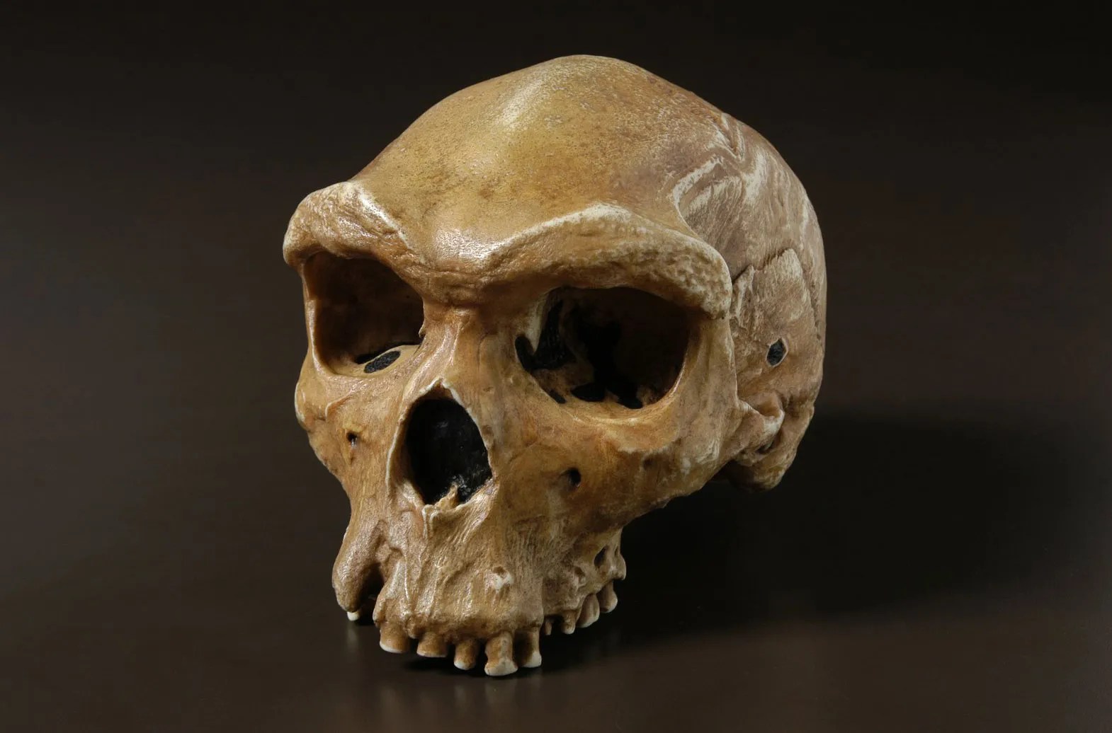
 and
and  , the number of matching bases is simply 2. Because mtDNA is circular, it’s not clear where to start the comparison. For example, we could start reading genome
  at the first
  , rather than the first base
  . However, the previous link demonstrates that there’s exactly one whole-genome alignment (otherwise known as a global alignment), or starting index for mtDNA, the rest of them are simply not credible for the reasons discussed above.
 , i.e., 90% of the genome, and retrieve all genomes that are at least a 90% match to Heidelbergensis. This produces the chart below, where the height of the bar provides the percentage of genomes in the applicable population that are at least a 90% match to the single Heidelbergensis genome. For example, 100% of the Iberian Romani are at least a 90% match to the Heidelbergensis genome, producing a height of 1.0 in the chart below. The population acronyms can be found at the back of [2], but just to highlight some of the obvious matches, KZ stands for Kazakhstan, IB stands for Iberian Romani, IT stands for Italy, and RU stands for Russia.
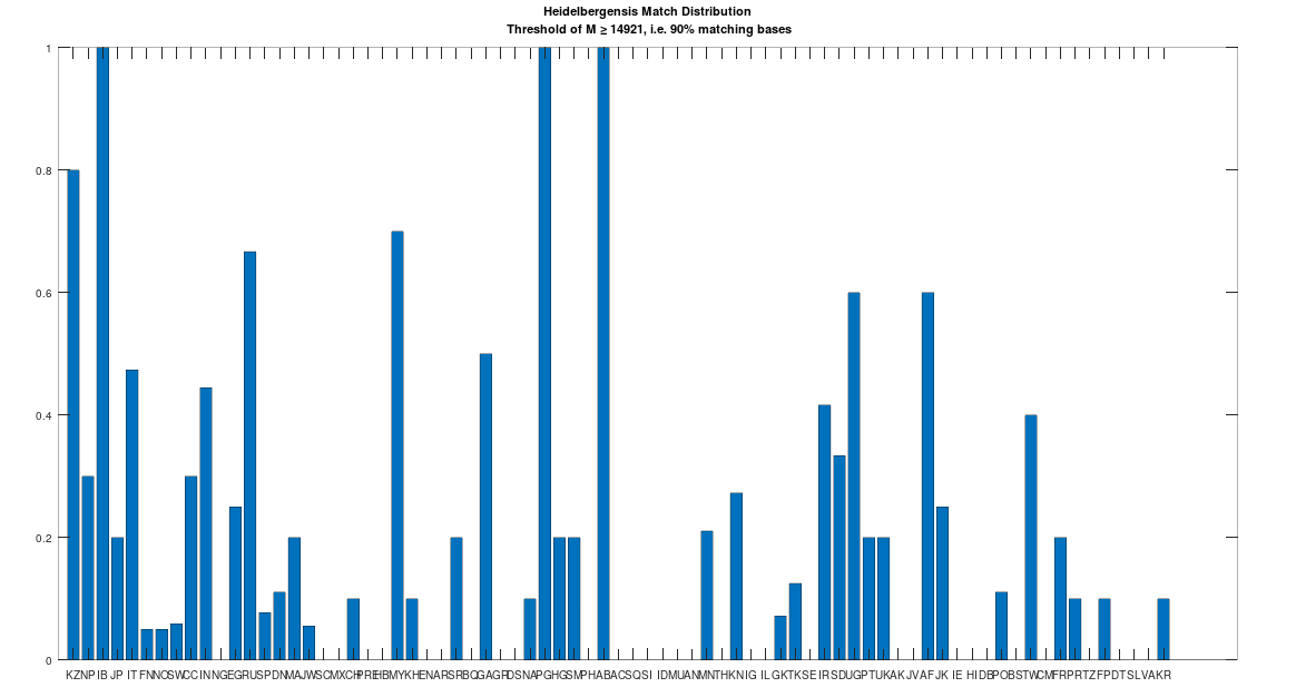
 . That is, at each base, we have two random variables, one for each genome, and each of those variables can take on a value of A, C, G, or T. If it’s truly random, then there are
  possible outcomes, and only 4 of those outcomes correspond to the bases being the same, producing a probability of
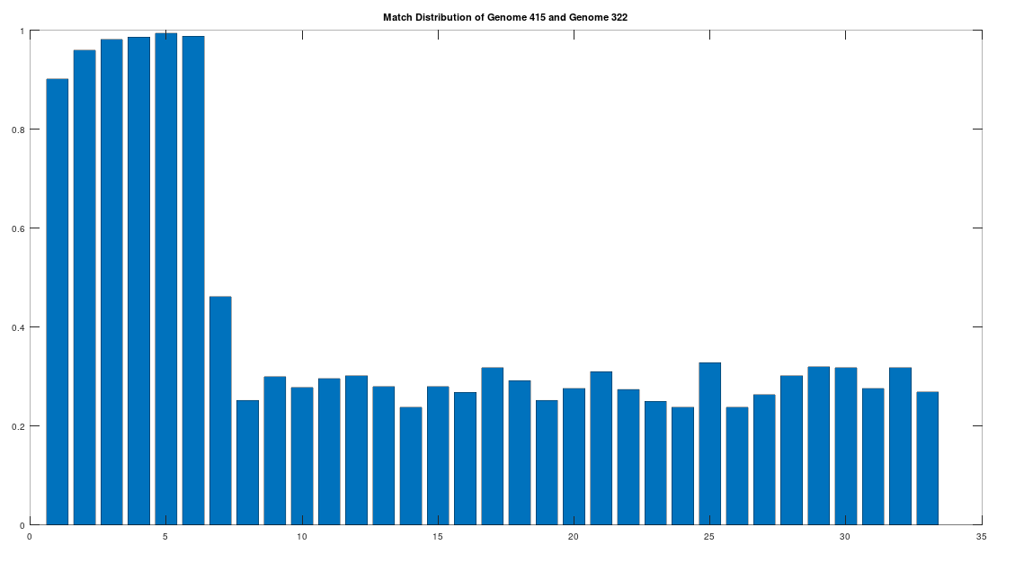
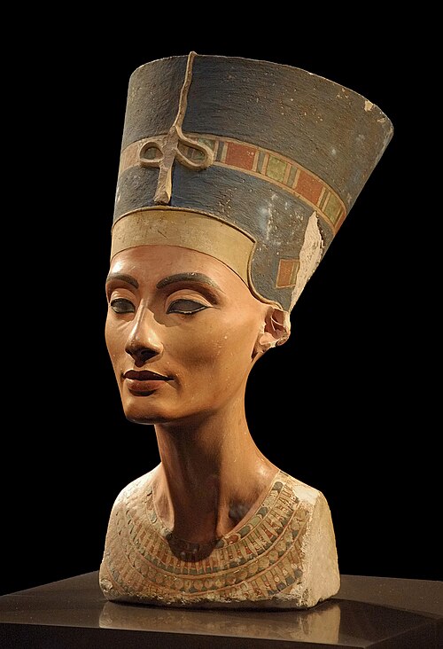
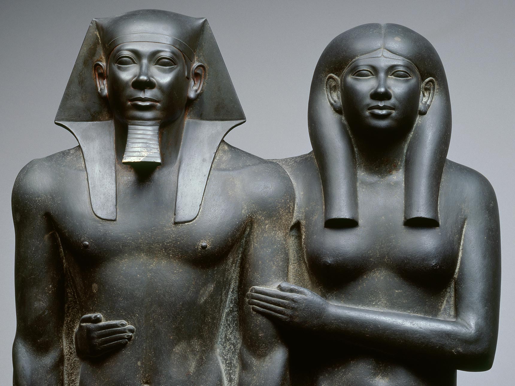
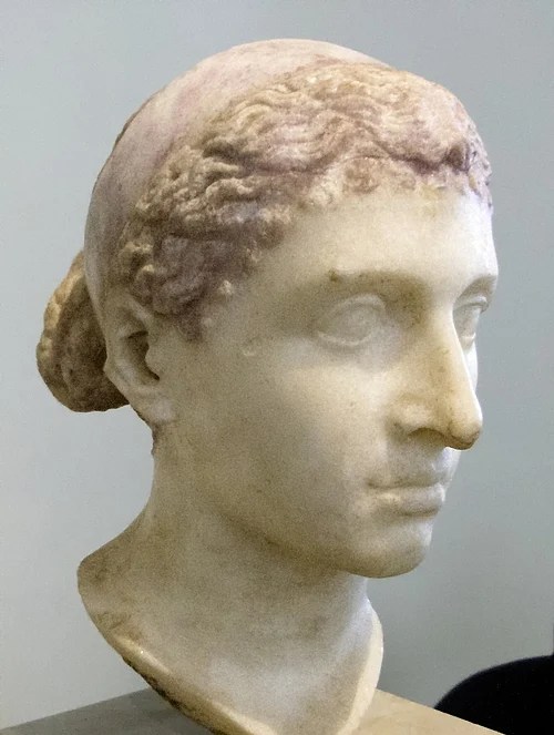
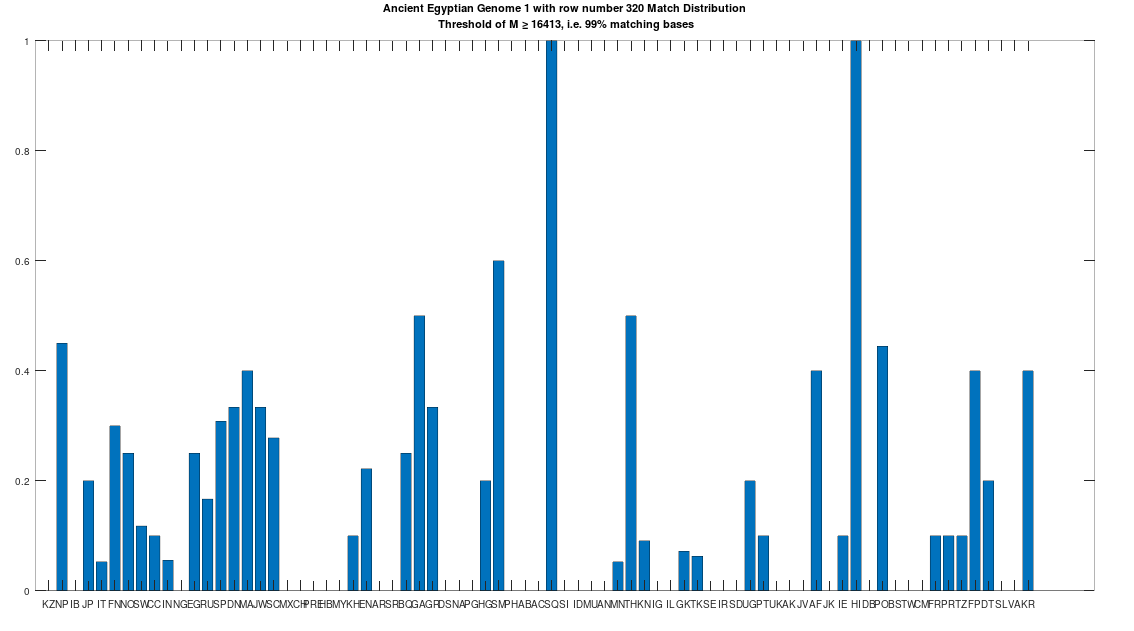
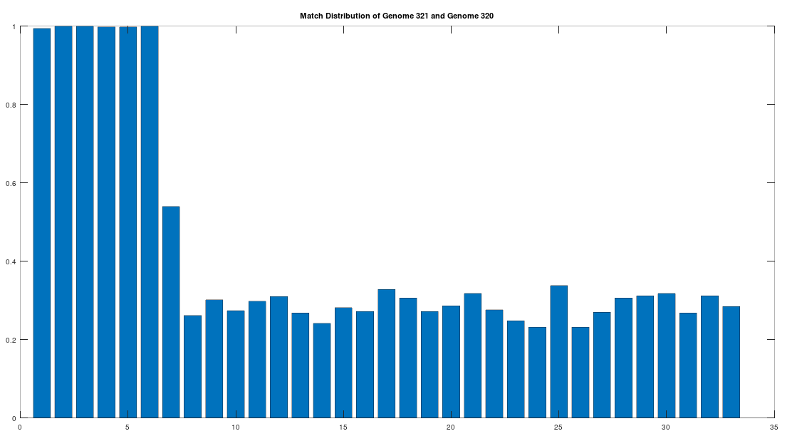
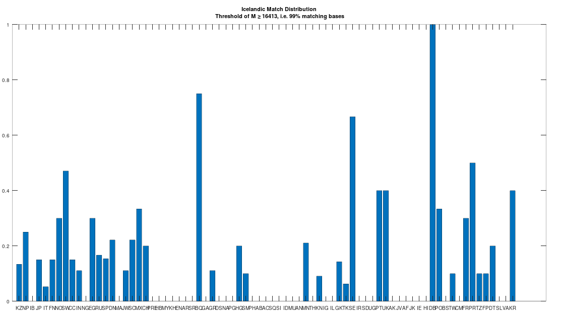
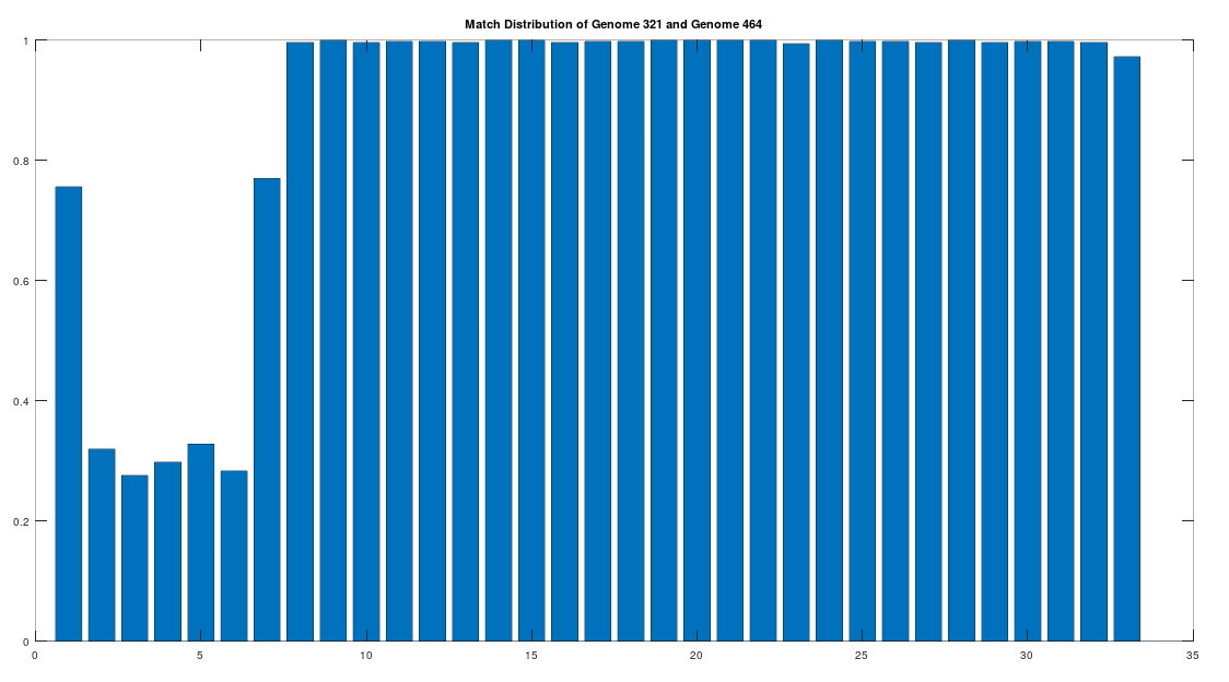
 and
and  . These two genomes have a match count of 3 bases, or 75% of the genome. Now let’s say we create an indel in genome
  , inserting a “G” after the first “A”, producing the genome
  . The match count is now instead 1 base, or 25% of the genome, depending on which genome’s length you use (i.e., 4 or 5).
 , a local alignment could, e.g., take the segment
  from
from  in genome
  mutations occurred over the entire history outlined above, which is not that many, since it spans around 500,000 years. Further, the local alignment algorithm found only 2 indels between the two genomes. This is all consistent with the extremely slow rate of mutation of mtDNA generally. That said, note that unlike the whole-genome algorithm, the local alignment algorithm is approximate, since there is (to my knowledge) no single segment length (in this case 500 bases) that is an objective invariant for comparing two genomes. Said otherwise, when using whole-genome comparison, both mathematical theory and empiricism show there’s only one global alignment, and therefore only one algorithm that gets the job done. In contrast, local alignments can produce different results if we vary the segment length, which is again in this case set to 500 bases. But the bottom line is, there really isn’t that much change over a huge period of time.
 and
and  . If we count matching bases using the first index of each genome, then the number of matching bases is zero. If instead we start at the first index of
  and the second index of
  (and loop back around to the first ‘G’ of
  and
and  . First you’ll note these genomes are not the same length, unlike in the example above, which is another factor to be considered when developing an alignment for comparison. If we simply use the first three bases of each genome for comparison, then the match count will be one, since the first two initial ‘A’s match. If instead we use index two of
  , then the entire
  sequence matches, and the resultant match count will be three.
 . As for accuracy, using Nearest Neighbor to predict the ethnicity of each individual in my dataset produces an accuracy of 30.87%, and because there are 75 global ethnicities, chance implies an accuracy of
  . As such, we can conclude that the Nearest Neighbor algorithm is not producing random results, and more generally, produces results that provide meaningful information about the ethnicities of individuals based solely upon their mtDNA, which is remarkable, since ethnicity is a complex trait, that clearly should depend upon paternal ancestry as well.
 of Norwegian genomes map to Pashtuns, who are
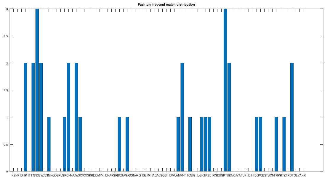
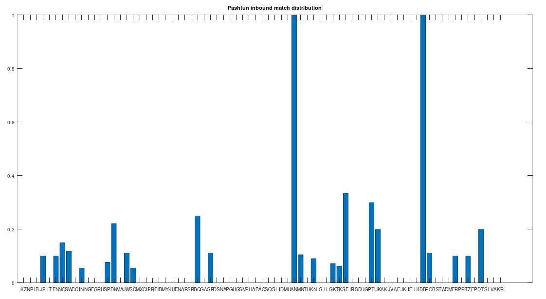
 , so these are plainly meaningful, nearly identical matches. Finally, these Pashtun genomes that are turning up as Nearest Neighbors are heterogeneous. That is, it’s not the case that a single Pashtun genome is popping up globally, and instead, multiple distinct Pashtun genomes are popping up globally as Nearest Neighbors. One not-so-plausible explanation that I think should be addressed is the
  sequences of bases of length 15, since there are 4 possible bases, ACGT. We want to know how likely it is that we find a given fixed sequence of length 15, anywhere in the mtDNA genome. If we find it more than once, that’s great, we’re just interested initially in the probability of finding it at least once. The only case that does not satisfy this criteria, is the case where it’s not found at all. The probability of two random 15 base sequences successfully matching at all 15 bases is
  . Note that a full mtDNA genome contains
  bases. As such, we have to consider comparing 15 bases starting at any one of the
  indexes available for comparison, again considering all cases where it’s found at least once as a success.
 , the probability of failure at a given index is
  . Therefore, the probability that we find zero matches over all
  , and so the probability that we find at least one match is given by
  . That’s a pretty small probability, so we should already be impressed that we find this specific sequence of 15 bases in basically all human mtDNA genomes in the dataset.

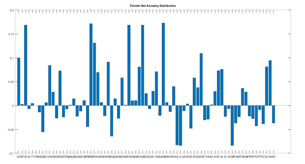
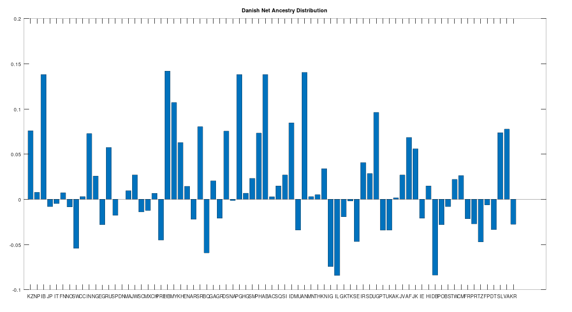


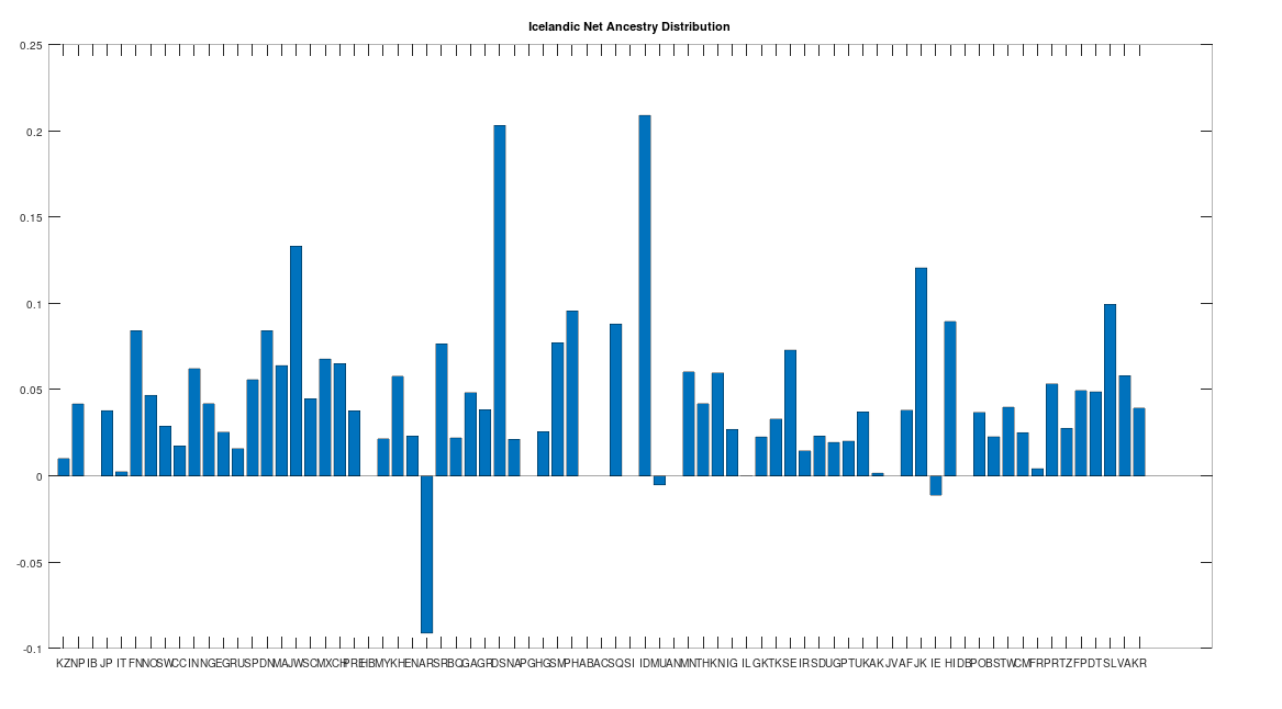
 calculations, all done on a consumer device. I’d wager professional computers can now start to tackle much larger genomes using similar techniques. As a result, I think we’re going to find that a lot of people contain a lot of truly archaic DNA generally. Any argument to the contrary is sort of strange, because if people stopped selecting archaic female mates, then archaic mtDNA should have vanished, and it obviously didn’t, leading to the conclusion, that the rest of the genome likely does contain archaic DNA generally.