Human Migration and mtDNA

January 7, 2026January 7, 2026 / erdosfan / Leave a comment

Genetic Alignment

Because of relatively recent advances in genetic sequencing, we can now read entire mtDNA genomes. However, because mtDNA is circular, it’s not clear where you should start reading the genome. As a consequence, when comparing two genomes, you have no common starting point, and the selection of that starting point will impact the number of matching bases. As a simple example, consider the two fictitious genomes $x = (A,C,A,G)$ and $y = (G,A,C,A)$ . If we count matching bases using the first index of each genome, then the number of matching bases is zero. If instead we start at the first index of $x$ and the second index of $y$ (and loop back around to the first ‘G’ of $y$ ), the match count will be four, or 100% of the bases. As such, determining the starting indexes for comparison (i.e., the genome alignment) is determinative of the match count.

It turns out that mtDNA is unique in that it is inherited directly from the mother, generally without any mutations at all. As such, the intuition for combinations of sequences typically associated with genetics is inapplicable to mtDNA, since there is no combination of traits or sequences inherited from the mother and the father, and instead a basically perfect copy of the mother’s genome is inherited. As a result, it makes perfect sense to use a global alignment, which we did above, where we compared one entire genome $x$ to another entire genome $y$ . In contrast, we could instead make use of a local alignment, where we compare segments of two genomes.

For example, consider genomes $A = (A,A,G,T)$ and $B = (A,G,T)$ . First you’ll note these genomes are not the same length, unlike in the example above, which is another factor to be considered when developing an alignment for comparison. If we simply use the first three bases of each genome for comparison, then the match count will be one, since the first two initial ‘A’s match. If instead we use index two of $A$ and index one of $B$ , then the entire $(A,G,T)$ sequence matches, and the resultant match count will be three.

Note that the number of possible global alignments is simply the length of the genome. That is, when using a global alignment, you “fix” one genome, and “rotate” the other, one base at a time, and that will cover all possible global alignments between the two genomes. In contrast, the number of local alignments is much larger, since you have to consider all local alignments of each possible length. As a result, it is much easier to consider all possible global alignments between two genomes, than local alignments. In fact, it turns out there is exactly one plausible global alignment for mtDNA, making global alignments extremely attractive in terms of efficiency. Specifically, it takes 0.02 seconds to compare a given genome to my entire dataset of roughly 650 genomes using a global alignment. Performing the same task using a local alignment takes one hour, and the algorithm I’ve been using considers only a small subset of all possible local alignments. That said, local alignments allow you to take a closer look at two genomes, and find common segments, which could indicate a common evolutionary history. This note discusses global alignments, I’ll write something soon that discusses local alignments, as a second look to support my work on mtDNA generally.

Nearest Neighbor

The Nearest Neighbor algorithm can provably generate perfect accuracy for certain Euclidean datasets. That said, DNA is obviously not Euclidean, and as such, the results I proved do not hold for DNA datasets. However, common sense suggests we might as well try it, and it turns out, you get really good results that are significantly better than chance. To apply the Nearest Neighbor algorithm to an mtDNA genome $x$ , we simply find the genome $y$ that has the most bases in common with $x$ , i.e., its best match in the dataset, and hence, its “Nearest Neighbor”. Symbolically, you could write $y = NN(x)$ . As for accuracy, using Nearest Neighbor to predict the ethnicity of each individual in my dataset produces an accuracy of 30.87%, and because there are 75 global ethnicities, chance implies an accuracy of $\frac{1}{75} = 1.3\%$ . As such, we can conclude that the Nearest Neighbor algorithm is not producing random results, and more generally, produces results that provide meaningful information about the ethnicities of individuals based solely upon their mtDNA, which is remarkable, since ethnicity is a complex trait, that clearly should depend upon paternal ancestry as well.

The Global Distribution of mtDNA

It turns out the distribution of mtDNA is truly global, and a result, we should not be surprised that the accuracy of the Nearest Neighbor method as applied to my dataset is a little low, though as noted, it is significantly higher than chance and therefore plainly not producing random predictions. That is, if we ask what is e.g., the best match for a Norwegian genome, you could find that it is a Mexican genome, which is in fact the case for this Norwegian genome. Now you might say this is just a Mexican person that lives in Norway, but I’ve of course thought of this, and each genome has been diligenced to ensure that the stated ethnicity of the person is e.g., Norwegian.

Now keep in mind that this is literally the closest match for this Norwegian genome, and it’s somehow on the other side of the world. But high school history teaches us about migration over the Bering Strait, and this could literally be an instance of that, but it doesn’t have to be. The bottom line is, mtDNA mutates so slowly, that outcomes like this are not uncommon. In fact, by definition, because the accuracy of the Nearest Neighbor method is 38.07% when applied to predicting ethnicity, it must be the case that 100% – 38.07% = 69.13% of genomes have a Nearest Neighbor that is of a different ethnicity.

One interpretation is that, oh well, the Nearest Neighbor method isn’t very good at predicting ethnicity, but this is simply incorrect, because the resultant match counts are almost always over 99% of the entire genome. Specifically, 605 of the 664 genomes in the dataset (i.e., 91.11%) map to a Nearest Neighbor that is 99% or more identical to the genome in question. Further, 208 of the 664 genomes in the dataset (i.e., 31.33%) map to a Nearest Neighbor that is 99.9% or more identical to the genome in question. The plain conclusion is that more often than not, nearly identical genomes are found in different ethnicities, and in some cases, the distances are enormous.

In particular, the Pashtuns are the Nearest Neighbors of a significant number of global genomes. Below is a chart showing the number of times (by ethnicity) that a Pashtun genome was a Nearest Neighbor of that ethnicity. So e.g., returning to Norway (column 7), there are 3 Norwegian genomes that have a Pashtun Nearest Neighbor, and so column 7 has a height of 3. More generally, the chart is produced by running the Nearest Neighbor algorithm on every genome in the dataset, and if a given genome maps to a Pashtun genome, we increment the applicable column for the genome’s ethnicity (e.g., Norway, column 7). There are 20 Norwegian genomes, so $\frac{3}{20} = 15\%$ of Norwegian genomes map to Pashtuns, who are generally located in Central Asia, in particular Afghanistan. This seems far, but in the full context of human history, it’s really not, especially given known migrations, which covered nearly the whole planet.

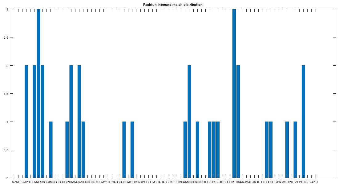
The chart above is not normalized to show percentages, and instead shows the integer number of Pashtun Nearest Neighbors for each column. However, it turns out that a significant percentage of genomes in ethnicities all over the world map to the Pashtuns, which is just not true generally of other ethnicities. That is, it seems the Pashtuns are a source population (or closely related to that source population) of a significant number of people globally. This is shown in the chart below, which is normalized by dividing each column by the number of genomes in that column’s population, producing a percentage.

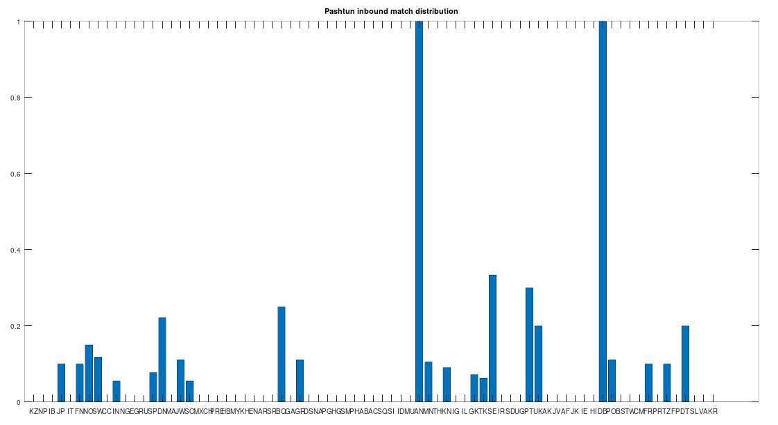
As you can see, a significant percentage of Europeans (e.g., Finland, Norway, and Sweden, columns 6, 7, and 8 respectively), East Asians (e.g., Japan and Mongolia, columns 4 and 44, respectively), and Africans (e.g., Kenya and Tanzania, columns 46 and 70, respectively), have genomes that are closest to Pashtuns. Further, the average match count to a Pashtun genome over this chart is $99.75\%$ , so these are plainly meaningful, nearly identical matches. Finally, these Pashtun genomes that are turning up as Nearest Neighbors are heterogeneous. That is, it’s not the case that a single Pashtun genome is popping up globally, and instead, multiple distinct Pashtun genomes are popping up globally as Nearest Neighbors. One not-so-plausible explanation that I think should be addressed is the Greco-Bactrian Kingdom, which overlaps quite a bit with the geography of the Pashtuns. The hypothesis would be that Ancient Greeks brought European mtDNA to the Pashtuns. Maybe, but I don’t think Alexander the Great made it to Japan, so we need a different hypothesis to explain the global distribution of Pashtun mtDNA.

All of this is instead consistent with what I’ve called the Migration-Back Hypothesis, which is that humanity begins in Africa, migrates to Asia, and then migrates back to Africa and Europe, and further into East Asia. This is a more general hypothesis that many populations, including the Pashtuns, migrated back from Asia to Africa and Europe, and extended their presence into East Asia. The question is, can we also establish that humanity began in Africa using these and other similar methods? Astonishingly, the answer is yes, and this is discussed at some length in a summary on mtDNA that I’ve written.

Early Machine Learning Innovations

September 28, 2025September 28, 2025 / erdosfan / Leave a comment

I’m certainly not a scholar on the topic, but I am interested in the history of Machine Learning, and this morning, I discovered a concept known as the Fisher Information. This is the same Sir Ronald Fisher that developed the Iris Dataset in 1936, which is most certainly a Machine Learning dataset, though it predates the first true computer the ENIAC which was built in 1945. The point being that the Iris Dataset itself is way ahead of its time, using measurable characteristics of various flowers to then determine the species of the flowers. This is a deep idea, in that you have the mathematical classification of species, which I would argue goes beyond the anatomical, and brings biology into the mathematical sciences.

But on top of this, and what seem to be many other achievements I don’t know much about, he had a really clever idea regarding mutual information between variables. Specifically, how much does a given probability distribution $f(X,\theta)$ change as a function of $\theta$ . His answer was to look at the derivative of $f$ as a function of $\theta$ , though the specific formula used is a bit more complicated. Nonetheless, the basic idea is, how sensitive is a distribution to one of its parameters, and what does that tell me.

This is exactly what Machine Learning engineers do all the time, which is to test the relevance of a dimension. Just imagine you had a dataset with dimensions $1$ through $N$ , and that you have a prediction function on that dataset $F(x_1, \ldots, x_N)$ . Now imagine you add a set of weights $(\theta_1, \ldots \theta_N)$ , for $\theta_i \in [0,1]$ , so that you instead consider the function $F(\theta_1 x_1, \ldots, \theta_N x_N)$ . That is, we’ve added weights that will reduce the contribution of each dimension simply by multiplying by a constant in $[0,1]$ . This is one of the most basic things you’ll learn in Machine Learning, and the rate of change in accuracy as a function of each $\theta_i$ will provide information about how important each dimension is to the prediction function. This is basically what Fisher did, except almost one hundred years ago, effectively discovering a fundamental tool of Machine Learning.

The point is more than just historical, I think Machine Learning is a buzzword used to cover up the fact that a lot of this stuff was known a long time ago, and that Artificial Intelligence is, generally speaking, far more advanced than the public realizes, and that as a matter of logical implication, most of what we believe to be new and exciting breakthroughs are often mundane adaptations of existing methods and technology. The fact that so much money is being poured into the market is disturbing, because I have no idea what these people do all day.

Note on Ramsey’s Theorem

October 28, 2024October 28, 2024 / erdosfan / Leave a comment

It’s always bothered me that Ramsey’s Theorem is not probabilistic. For example, R(3,3), i.e., the smallest order complete graph that contains either a complete graph on 3 vertices, or an empty graph on 3 vertices, is 6. This means that literally every graph with 6 or more vertices contains either a complete graph on e vertices, or an empty graph on e vertices. This is not probabilistic, because it’s simply true, for all graphs on 6 or more vertices. But it just dawned on me, you can construct a probabilistic view of this fact, which is that on fewer than 6 vertices, the probability is less than one, whereas with 6 or more vertices, the probability is 1. This is true in the literal sense, since less than all graphs with fewer than 6 vertices have a complete graph on 3 vertices, or an empty graph on 3 vertices, but some will. I think this could actually be quite deep, and connect to random graphs, but I need some time to think about it.

Another thought, that I think I’ve expressed before, if we can analogize Ramsey’s Theorem to time, then it would imply that certain structures eventually become permanent. This is a truly strange idea, and though I’m just brain storming, intuitively, it doesn’t sound wrong. And now that I’ve thought a bit more about it, I’ve definitely had this idea before:

Specifically, correlation between two random variables can be thought of as an edge between two vertices, where the vertices represent the variables, and the edge represents the presence or absence of correlation. If we consider all random variables together, then it’s clear that having no correlation at all would correspond to an empty graph, and correlation between all variables would correspond to a complete graph. If all graphs are equally likely, no correlation, and total correlation would be equally likely, and in fact the least likely possibilities for any graph with more than two vertices (when compared to at least some but less than total correlation). As a result, if we randomly select, random variables, we should generally find at least some correlation, regardless of their nature or apparent relationships.

If we imagine time quantized on a line, with a vertex representing a moment, and allow for one moment in time to be related to another moment in time by connecting them with an edge, we will have a graph, that just happens to be visualized along a line. Applying Ramsey Theory, we know that certain structures must emerge over time, since we are allowing for the possibility of ever larger graphs. At the same time, the correlation argument above implies that each moment should have some possibly non-causal connection to other moments, producing non-empty graphs. That is, if one moment is connected to another in the remote past, it’s really not credible that it’s causal, and is instead an artifact of this line of thinking. This argument as a whole implies the possibility that reality has non-causal relationships over time, regardless of whether or not the past, present, or future, is memorialized in any way, and regardless of whether or not the past, present, or future is physically real, because these are immutable, abstract, arguments. All of that said, this is a lot to think about, and I need to organize it a bit more, but the core idea seems sound, and that’s disturbing.

Spatial Uncertainty and Order

September 28, 2024September 28, 2024 / erdosfan / Leave a comment

I presented a measure of spatial uncertainty in my paper, Sorting, Information, and Recursion [1], specifically, equation (1). I proved a theorem in [1] that equation (1) is maximized when all of its arguments are equal. See, Theorem 3.2 of [1]. This is really interesting, because the same is true of the Shannon Entropy, which is maximized when all probabilities are equal. They are not the same equation, but they’re similar, and both are rooted in the logarithm. However, my equation takes real number lengths or vectors as inputs, whereas Shannon’s equations takes probabilities as inputs.

I just realized, that Theorem 3.2 in [1], implies the astonishing result, that the order of a set of observations, impacts the uncertainty associated with those observations. That is, we’re used to taking a set of observations, and ignoring the ordinal aspect of the data, unless it’s explicitly a time series. Instead, Theorem 3.2 implies that the order in which the data was generated is always relevant in terms of the uncertainty associated with the data.

This sounds crazy, but I’ve already shown empirically, that these types of results in information theory work out in the real world. See, Information, Knowledge, and Uncertainty [2]. The results in [2], allow us to take a set of classification predictions, and assign a confidence value to them, that are empirically correct, in the sense that accuracy increases as a function of confidence. The extension here, is that spatial uncertainty is also governed by an entropy-type equation, specially equation (1), which is order dependent. We could test this empirically, by simply measuring whether or not prediction error, is actually impacted by order, in an amount greater than chance. That is, we filter predictions, as a function of spatial uncertainty, and test whether or not prediction accuracy improves as we decrease uncertainty.

Perhaps most interesting, because equation (1) is order dependent, if we have an observed uncertainty for a dataset (e.g., implied from prediction error), and we for whatever reason do not know the order in which the observations were made, we can then set equation (1) equal to that observed uncertainty, and solve for potential orderings that produce values approximately equal to that observed uncertainty. This would allow us to take a set of observations, for which the order is unknown, and limit the space of possible orderings, given a known uncertainty, which can again be implied from known error. This could allow for implications regarding order that exceed a given sample rate. That is, if our sample rate is slower than the movement of the system we’re observing, we might be able to restrict the set of possible states of the system using equation (1), thereby effectively improving our sample rate in that regard. Said otherwise, equation (1) could allow us to know about the behavior of a system between the moments we’re able to observe it. Given that humanity already has sensors and cameras with very high sample rates, this could push things even further, giving us visibility into previously inaccessible fractions of time, perhaps illuminating the fundamental unit of time.

Bilateral Comparison of Ancestry Flows

May 30, 2024 / erdosfan / Leave a comment

In a previous note, I presented an algorithm that allows you to test ancestry flows between three populations. The method in the previous note already allows for bilateral comparisons, between the three populations. However, if you repeatedly apply the trilateral test, using all possible triplets from a dataset of populations, you will produce a graph. This graph will have bilateral flows using information derived from the entire dataset, as opposed to just three populations.

I’m still mulling through the data, but in the previous note, I stated that Norway seems to be the root population for basically everyone. I now think it’s somewhere around Holland and Denmark, using the full graph produced by the algorithm below. This is not to undermine the hypothesis that human life began in Africa, instead, the hypothesis is that modern homosapiens seem to have emerged pretty recently, in Northern Europe. All of this stuff needs to be squared off with other known results, in particular archeological results, but it does explain how, e.g., South East Asians have the gene for light skin, by descendancy (i.e., they’re the ancestors of white Europeans). I’m merely expanding the claim, pointing out that a lot of Africans also test as the descendants of Europeans, using mtDNA.

Here’s the code, more to come. You just call it from the command line saying “graph_matrix = generate_full_ancestry_graph(dataset, num_classes, N);”. The resultant graph flows are stored in graph_matrix. You’ll need the rest of the code, which is included in the paper I link to in the previous note.

generate_full_ancestry_graph Download

generate_ancestry_graph Download

mtDNA and IQ

February 17, 2024February 18, 2024 / erdosfan / Leave a comment

Introduction

I’ve noticed in the past that Finns have significantly higher IQ’s than the Swedes and Norwegians. This is in my opinion the group of people to study if you’re interested in the nature of intelligence, because they’re all very similar people, from roughly equally rich nations, in the same part of the world, which should allow innate ability to take control. One notable difference is that the Finns speak an Uralic language, whereas the Norwegians and Swedes speak a Germanic language. There could be something to this, but investigating the problem again today led me to what seems an inescapable conclusion, that whatever the connection is between mtDNA and intelligence, it simply cannot account for the distribution of IQ as it exists.

Instead I now believe that brain structure is the most important factor in intelligence, which simply cannot be controlled by mtDNA in any credible way. Specifically, my thinking is rooted in algorithmic complexity, that if you have two equally powered machines, running different algorithms that accomplish the same task, then the machine with the more efficient algorithm of the two will be the most powerful of the two. Translated to biology, if you have two brains that both consume the same amount of power per unit of time, and have the same “clock rate”, one brain could still be vastly more powerful than the other, due simply to different structure. This could explain e.g., the fact that some birds can talk, whereas some dogs will eat until they vomit, despite the fact that birds have brain volumes that are a small fraction of a dog’s brain volume.

mtDNA and Intelligence

Despite the apparent complexity of the subject, this is going to be a short note, because the idea that mtDNA controls for IQ is apparently nonsense, despite the scholarship on the topic (not picking on anyone, but here’s a decent article that runs through some credible arguments for the role of mtDNA in intelligence). But as you’ll see, whole-genome sequencing throws the argument in the garbage.

There’s no nice way to say this, but the Roma people have pretty low IQs, but what’s most interesting about them, is that they are basically identical to each other, and all other people of that maternal line, including about 100% of Papuans, 67% of Russians, and about 30% of Taiwanese people. If you want to test the results yourself, you can see my paper, “A New Model of Computational Genomics” [1], which includes all the software, and a detailed walkthrough to explain how I end up with these numbers. At a high level, the Papuans, Russians, and Taiwanese people in this group of Roma lineage, are all a 99% match to the Iberian Roma, with respect to their mtDNA. If mtDNA controlled intelligence, then all of those populations should have similarly low IQ’s, since they’re basically identical to the Roma. This is just not true, and instead the Taiwanese have around the highest and second highest IQ on Earth, and the Russians have roughly the same IQ as the Norwegians and Swedes, despite the fact that Russia is, quite frankly, poor and dysfunctional compared to Norway and Sweden.

One important note, though you’ll often hear that “humans are 98% monkey”, or some nonsense like that, the algorithms in [1] use what’s called a global alignment, and as a consequence, they’re extremely sensitive to changes in position, causing e.g., the Roma to have little more than chance in common with some people (i.e., about 25% of the mtDNA bases). This sensitivity is probably why the software in [1] is so powerful, and is able to predict ethnicity with about 80% accuracy, using mtDNA alone (which is pretty amazing). In contrast, NIH’s BLAST algorithm uses a local alignment, and so it deliberately seeks to maximize the number of matching bases, by shifting two genomes around, causing everyone to look the same, and therefore, throwing away valuable information about the genome.

Getting back to the core topic, if you pay attention to this limited set of facts, mtDNA is in the garbage as a driver of intelligence, and moreover, the role of poverty is not exactly clear either, since Russia is really poor compared to Norway and Sweden, and yet they have roughly the same IQs. So what is driving this? Cynically, I think IQ testing is really just testing for basic education (when you look at a map), which is absent in the truly poorest countries, but that doesn’t mean that we can’t debunk the connection between mtDNA and intelligence. But to be clear, I do think intelligence is genetic, and in anomalous cases like Finland, Cambodia, and Suriname, IQ becomes something interesting, because it’s at least a test. I just doubt it’s mtDNA driving the bus.

Some Answers from Computer Science

Even if we posit arguendo (which is not very nice) that there’s something wrong with Roma mtDNA, this would simply imply that they have low energy per unit of time, perhaps as a function of fixed caloric intake and environment. To make this less abstract, let’s fix a Norwegian guy (not Roma) and a Russian guy (Roma), and give them the same food, education, climate, environment, clothes, etc., over a lifetime. Under this assumption, the Russian guy will produce less energy over his lifetime, and therefore, his brain has a lower output. But this is garbage as an argument, for mechanical reasons: if the Russian guy has a more efficient brain, then he doesn’t need as much power to run his brain. As a consequence, his output over a lifetime could in fact be higher.

To make things completely concrete, if you use a brute force method to sort a list of 10 letters, you’ll have to perform 10! = 3,628,800 calculations. If you instead use my parallel method, you’ll have to make between 3 and 4 calculations. As you can plainly see, there is an ocean between these two approaches to solving even the simple problem of sorting a list. As a consequence, the most sensible answer is, in my opinion, that brain structure controls for intelligence, for the simple reason, that it encodes the algorithms we use to solve the problems we face every day. Some people have fast ones, some people have dumb ones, and then there’s (probably) most people in the middle.

Returning to the birds versus dogs analogy, I think it’s not ridiculous to argue that birds have vastly more efficient brains than dogs, that something along the lines of computational efficiency is taking place in the brain of a bird, that allows it to perform complex tasks, with a smaller, presumably lower-energy brain. For the same reasons, this could explain the obvious fact that some people are wildly more intelligent than others, despite (possibly) having the same maternal line. Because intelligence varies within a given ethnicity, I can tell you that you are e.g., Norwegian, with high accuracy using just your mtDNA, but there’s no way of knowing (to my knowledge) whether you’re one of the dumb ones. This doesn’t preclude identifying deficiencies in mtDNA that will make you dangerously ill, and therefore not very bright, but it just doesn’t make sense that the means of power-production controls the most complex structure in the Universe –

It’s a single bean, in an ocean of genetic information.

Information Overload

artificial-intelligence