Genetic Alignment
Because of relatively recent advances in genetic sequencing, we can now read entire mtDNA genomes. However, because mtDNA is circular, it’s not clear where you should start reading the genome. As a consequence, when comparing two genomes, you have no common starting point, and the selection of that starting point will impact the number of matching bases. As a simple example, consider the two fictitious genomes 


It turns out that mtDNA is unique in that it is inherited directly from the mother, generally without any mutations at all. As such, the intuition for combinations of sequences typically associated with genetics is inapplicable to mtDNA, since there is no combination of traits or sequences inherited from the mother and the father, and instead a basically perfect copy of the mother’s genome is inherited. As a result, it makes perfect sense to use a global alignment, which we did above, where we compared one entire genome
For example, consider genomes 


Note that the number of possible global alignments is simply the length of the genome. That is, when using a global alignment, you “fix” one genome, and “rotate” the other, one base at a time, and that will cover all possible global alignments between the two genomes. In contrast, the number of local alignments is much larger, since you have to consider all local alignments of each possible length. As a result, it is much easier to consider all possible global alignments between two genomes, than local alignments. In fact, it turns out there is exactly one plausible global alignment for mtDNA, making global alignments extremely attractive in terms of efficiency. Specifically, it takes 0.02 seconds to compare a given genome to my entire dataset of roughly 650 genomes using a global alignment. Performing the same task using a local alignment takes one hour, and the algorithm I’ve been using considers only a small subset of all possible local alignments. That said, local alignments allow you to take a closer look at two genomes, and find common segments, which could indicate a common evolutionary history. This note discusses global alignments, I’ll write something soon that discusses local alignments, as a second look to support my work on mtDNA generally.
Nearest Neighbor
The Nearest Neighbor algorithm can provably generate perfect accuracy for certain Euclidean datasets. That said, DNA is obviously not Euclidean, and as such, the results I proved do not hold for DNA datasets. However, common sense suggests we might as well try it, and it turns out, you get really good results that are significantly better than chance. To apply the Nearest Neighbor algorithm to an mtDNA genome 

The Global Distribution of mtDNA
It turns out the distribution of mtDNA is truly global, and a result, we should not be surprised that the accuracy of the Nearest Neighbor method as applied to my dataset is a little low, though as noted, it is significantly higher than chance and therefore plainly not producing random predictions. That is, if we ask what is e.g., the best match for a Norwegian genome, you could find that it is a Mexican genome, which is in fact the case for this Norwegian genome. Now you might say this is just a Mexican person that lives in Norway, but I’ve of course thought of this, and each genome has been diligenced to ensure that the stated ethnicity of the person is e.g., Norwegian.
Now keep in mind that this is literally the closest match for this Norwegian genome, and it’s somehow on the other side of the world. But high school history teaches us about migration over the Bering Strait, and this could literally be an instance of that, but it doesn’t have to be. The bottom line is, mtDNA mutates so slowly, that outcomes like this are not uncommon. In fact, by definition, because the accuracy of the Nearest Neighbor method is 38.07% when applied to predicting ethnicity, it must be the case that 100% – 38.07% = 69.13% of genomes have a Nearest Neighbor that is of a different ethnicity.
One interpretation is that, oh well, the Nearest Neighbor method isn’t very good at predicting ethnicity, but this is simply incorrect, because the resultant match counts are almost always over 99% of the entire genome. Specifically, 605 of the 664 genomes in the dataset (i.e., 91.11%) map to a Nearest Neighbor that is 99% or more identical to the genome in question. Further, 208 of the 664 genomes in the dataset (i.e., 31.33%) map to a Nearest Neighbor that is 99.9% or more identical to the genome in question. The plain conclusion is that more often than not, nearly identical genomes are found in different ethnicities, and in some cases, the distances are enormous.
In particular, the Pashtuns are the Nearest Neighbors of a significant number of global genomes. Below is a chart showing the number of times (by ethnicity) that a Pashtun genome was a Nearest Neighbor of that ethnicity. So e.g., returning to Norway (column 7), there are 3 Norwegian genomes that have a Pashtun Nearest Neighbor, and so column 7 has a height of 3. More generally, the chart is produced by running the Nearest Neighbor algorithm on every genome in the dataset, and if a given genome maps to a Pashtun genome, we increment the applicable column for the genome’s ethnicity (e.g., Norway, column 7). There are 20 Norwegian genomes, so 
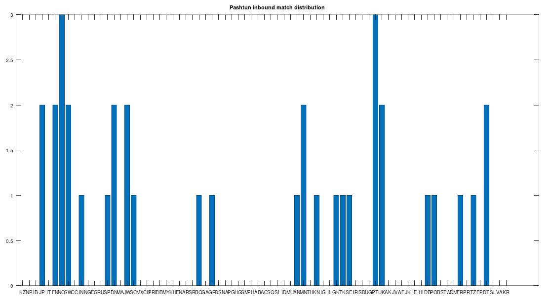
The chart above is not normalized to show percentages, and instead shows the integer number of Pashtun Nearest Neighbors for each column. However, it turns out that a significant percentage of genomes in ethnicities all over the world map to the Pashtuns, which is just not true generally of other ethnicities. That is, it seems the Pashtuns are a source population (or closely related to that source population) of a significant number of people globally. This is shown in the chart below, which is normalized by dividing each column by the number of genomes in that column’s population, producing a percentage.
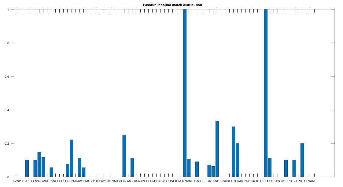
As you can see, a significant percentage of Europeans (e.g., Finland, Norway, and Sweden, columns 6, 7, and 8 respectively), East Asians (e.g., Japan and Mongolia, columns 4 and 44, respectively), and Africans (e.g., Kenya and Tanzania, columns 46 and 70, respectively), have genomes that are closest to Pashtuns. Further, the average match count to a Pashtun genome over this chart is 
All of this is instead consistent with what I’ve called the Migration-Back Hypothesis, which is that humanity begins in Africa, migrates to Asia, and then migrates back to Africa and Europe, and further into East Asia. This is a more general hypothesis that many populations, including the Pashtuns, migrated back from Asia to Africa and Europe, and extended their presence into East Asia. The question is, can we also establish that humanity began in Africa using these and other similar methods? Astonishingly, the answer is yes, and this is discussed at some length in a summary on mtDNA that I’ve written.
 sequences of bases of length 15, since there are 4 possible bases, ACGT. We want to know how likely it is that we find a given fixed sequence of length 15, anywhere in the mtDNA genome. If we find it more than once, that’s great, we’re just interested initially in the probability of finding it at least once. The only case that does not satisfy this criteria, is the case where it’s not found at all. The probability of two random 15 base sequences successfully matching at all 15 bases is
  . Note that a full mtDNA genome contains
  bases. As such, we have to consider comparing 15 bases starting at any one of the
  indexes available for comparison, again considering all cases where it’s found at least once as a success.
 , the probability of failure at a given index is
  . Therefore, the probability that we find zero matches over all
  , and so the probability that we find at least one match is given by
  . That’s a pretty small probability, so we should already be impressed that we find this specific sequence of 15 bases in basically all human mtDNA genomes in the dataset.
 such that the output tape of
  contains the state of the Universe at time
  . That is, if we look at the output tape of
  , we will see a complete and accurate representation of the entire Universe at time
  , where
  is the state of the Universe excluding
  is the internal state of
  is the output tape of
  , which means that the output tape at time
  . This recurrence relation does not end, and as a consequence, if we posit the existence of such a machine, the output tape will contain the entire future of the Universe. This implies the Universe is completely predetermined.
 .
. and there is a one-to-correspondence
  . Further assume that the cardinality of
  , is not intuitively infinite, and as such, there is some
  , such that
  . Because
  is one-to-one, it must be the case that
  , but because
  such that
  . Because
  , but this contradicts the assumption that
  be some singleton. It would suffice to show that
  , since that would imply that there is a one-to-one correspondence from
  . Assume instead that
  . It must be the case that
  , since you can show there is
  , since removing a singleton from a countable set does not change its cardinality. Note we are allowing for infinite numbers that are capable of diminution by removal of a singleton arguendo for purposes of the proof. Analogously, it must be the case
  , since assuming
  would again imply that adding a singleton to a countable set would change its cardinality, which is not true. As such, because
  such that
  . That is, we can remove a subset from
  .
. , it must be the case that
  . However, on the lefthand side of the equation, the union over
  , which we’ve assumed to have a cardinality of less than
  , which completes the proof.
 .
. , which implies that,
 , and therefore,
 , and so
  .
. , and therefore,
  .
. . However, applying this produces a contradiction, specifically, we find that,
 , which implies that
  , and therefore
  .
. , which contradicts the assumption that
  that produces 1 cannot be 0, since we’ve shown that
  binary switches, the number of possible states is given by
  . That is, if we count all possible combinations of the set of switches, we find it is given by 2 raised to the power of the cardinality of the set. This creates a connection between the units of information, and cardinality. Let’s assume base 2 logarithms going forward. Specifically, if
  , has units of cardinality or number, and
  has units of bits. Though otherwise not relevant at the moment (i.e., there could be deeper connections), Shannon’s equation for Entropy also implies that the logarithm of a probability has units of bits. Numbers are generally treated as dimensionless, and so are probabilities, again implying that the logarithm always yields bits as its output.
 ? Physically, a system with one state cannot be used to meaningfully store information, since it cannot change states, and as such, the assumption that
  implies true results. Physically, the assertion that
  cannot be a real number, and has really unusual properties that nonetheless imply correct conclusions of mathematics.
 , it must be the case that
  . We can make sense of this by assuming that
  is defined over
  , other than at
  , and so
  , which implies that
  , and as such,
  . If we consider
  , we will find two correct results, depending how we evaluate the expression. If we evaluate what’s under the radical first, we have
  . If however we evaluate
  , we instead have
  , and so
  , where
  .
. , we have
  . Exponentiating, we find
  , but it suggests that
  is not dimensionless, though it is unitary.
 , Knowledge
  , and Uncertainty
  , as follows:
 .
. that can be known about the system, and so everything I know about the system
  , where
  and
and  and
and  and
and  , producing the following:
 , where
  ,
,  , and
, and  .
. and
and  and
and  . Because either could be a rational number, we must accept that rational cardinalities exist, given that the equation
  . As an example, let’s assume we’re considering a set of
  .
. possible states, and so your uncertainty has been reduced. However, because this information doesn’t change the underlying system in any way, and in general,
  , which is non-zero. We can then reasonably assume that
  states, and that
  . Now assume you’re told that all but one box has been eliminated as a possible location for the pebble. It follows that
  , and that
  . If
. If  , in the sense that all states are possible, and so our uncertainty is maximized, and our knowledge should be zero. However, if
  .
. change as a function of
  . His answer was to look at the derivative of
  through
  . Now imagine you add a set of weights
  , for
, for ![\theta_i \in [0,1]](https://s0.wp.com/latex.php?latex=%5Ctheta_i+%5Cin+%5B0%2C1%5D&bg=ffffff&fg=444444&s=0&c=20201002) , so that you instead consider the function
, so that you instead consider the function  . That is, we’ve added weights that will reduce the contribution of each dimension simply by multiplying by a constant in
 ![[0,1]](https://s0.wp.com/latex.php?latex=%5B0%2C1%5D&bg=ffffff&fg=444444&s=0&c=20201002) . This is one of the most basic things you’ll learn in Machine Learning, and the rate of change in accuracy as a function of each
. This is one of the most basic things you’ll learn in Machine Learning, and the rate of change in accuracy as a function of each  will provide information about how important each dimension is to the prediction function. This is basically what Fisher did, except almost one hundred years ago, effectively discovering a fundamental tool of Machine Learning.
 , which is less than
  . There is however no proof in that book of the general case, and instead only a proof of the finite case, expressed as a counting argument. I looked up proofs, and all the proofs I could find seem to have the same hole, which I’ll discuss.
 denote the power set of
  . That is, we are assuming arguendo that the cardinality of
  such that
  is surjective, which means that all elements of
  . That is, because we know
  . That said, a simple additional step will prove that we can always define
  , which will produce a non-empty set
  .
. . Because
  , there must be
  , such that
  , and
, and  . Because
  such that
  and
and  . If
. If  or
or  , then
  and
and  . Now define
  and
and  , but otherwise
  for
for  . If
. If  and
and  . If either is not a singleton (or both are not singletons), then it must be the case that either
  Note that
  such that
  . It must be the case that either
  or
or  . If
. If  , since by definition,
  . If
. If  , which completes the proof.
 , and let’s apply the proof above. Generally speaking, we would assume that the power set of the empty set contains one element, namely a set that contains the empty set as a singleton, represented as
  . Assuming we can even define
  . Because
  , it must be the case that
  . However, if we want
  , it must be the case that
  , even though
  , and instead,
  since
since  . That is, the accepted proof assumes
  , and let’s apply the proof above. The power set of a singleton is generally defined as
  . Because the accepted proof does not explicitly define
  . Because
  ,
,  . Again, the accepted proof fails.