Truly Derivative Dribble

Email: derivativedribble [at] yahoo [dot] com.

Twitter: My Profile

Friday June 26, 2009

My breakfast of choice

Friday May 29, 2009

My latest for the Atlantic: Could Government Intervention Help Markets Function Better?

Saturday May 16, 2009

My latest for the Atlantic: How NPR Mangled Geithner’s Plan For OTC Derivatives

Thursday May 7, 2009

My latest for the Atlantic: Boring Banking Will Not Save You

Friday May 1, 2009

My latest for the Atlantic: The Sorry State Of The Dismal Science

Thursday April 30, 2009

YOU MUST WATCH THIS: John Authers interviews Richard Thaler, behavorial economist and author of Nudge.

Friday April 17, 2009

My Latest for the Atlantic: Credit Default Swaps and Control Rights

Tuesday April 14, 2009

My latest for the Atlantic: The Art of the Banking Controversy

Friday April 10, 2009

My latest for the Atlantic: The Regulatory Pendulum and Electoral Guillotine

Wednesday April 8, 2009

My latest for the Atlantic

Friday April 3, 2009

Very nice chart from the FT on debt and demographics

Monday March 30, 2009

Recommended: FT interview with Obama

Friday March 27, 2009

Derivative Dribble on Twitter

My latest for the Atlantic Business

Wednesday March 25, 2009

High speed photos of exploding objects

Bank Executive’s home vandalized

MUST READ: Resignation letter of form AIGFP employee

HIGHLY RECOMMENDED: John Authers takes a look at the EMH and the future of wealth management

Friday March 20, 2009

HIGHLY RECOMMENDED: Washington Post takes us inside AIG-FP (“If they give back the money, then they will walk. And they will walk into the arms of AIG’s counterparties.”)

My latest for The Atlantic

HIGHLY RECOMMENDED: This Blog

Tuesday March 17, 2009

Fortune does a good job getting the facts straight about CDS

Friday March 13, 2009

Recommended: The Economist takes a look at credit markets

Berkshire downgraded by Fitch

Thursday March 12, 2009

Gates back on top as crisis wipes out other billionaires

Monday March 9, 2009

Hilarious

Friday March 6, 2009

Alpha Ville on the ocean of looming corporate defaults

Thursday March 5. 2009

Citi drops below $1

My latest for the Atlantic

Wednesday March 4, 2009

FDIC might go insolvent

Tuesday March 3, 2009

Derivatives market remains profitable business for J.P. Morgan

Very interesting data on the multiplier effect from the CBO

Tuesday February 24, 2009

My latest article for the Atlantic

Monday February 23, 2009

HIGHLY RECOMMENDED: Howard Davies, head of LSE and former FSA Chairman, on bank regulation

FT on the prospect of a depression in Spain

Rick Santelli rouses traders over Obama’s housing plan

Sunday February 22, 2009

Citi in talks with U.S. Government over common equity stake

Thursday February 19, 2009

Must read: Buiter rips apart Obama’s housing plan

Saturday February 14, 2009

Collective decision making in animals and humans

Thursday February 12, 2009

New York edges closer to expanding rent control

Wednesday February 11, 2009

Rep. Kanjorski tells us how close to the edge we were

Treasury’s 6 and a half page plan to save the world

Tuesday February 10, 2009

Great article by the FT’s John Authers on the prospects of an equity bounce-back

Friday February 5, 2009

U.S. cuts almost 600,000 jobs

Wednesday February 4, 2009

My latest article for the Atlantic Business Channel

Tuesday February 3, 2009

E.U. pushes CDS exchange

Monday February 2, 2009

For my fellow music lovers: Classic Arts Showcase on YouTube

Consumers turn to thrift

Unemployment hits China

S&P says 200 defaults expected

Thursday January 30, 2009

Crash like this expected only once over next 34,000 years

Contraction bad, but better than expected

Wednesday January 28, 2009

John Authors on the perception of a bargain

Capacity drops in France and Italy

World growth worst in 60 years

Tuesday January 27, 2009

Japanese CDS spreads widen

The original Carlo Ponzi

Madoff Jr. gets busted in $400 million Ponzi scheme

Great article from Atlantic’s new business section

Monday January 26, 2009

Iceland’s government tumbles under pressure

Unemployment rate looms over banking sector

Redemptions slam hedge funds

Wednesday January 23, 2009

Obama thinks stimulus package could be ready mid February

Muni derivatives under investigation

Cocoa prices on the move

Very interesting John Authers video on the prospect of a slow down in China

Pope goes digital

U.K. officially in a recession

Wednesday January 22, 2009

Google beats the heard

N.Y. Times provides some perspective on the severity of the crisis

U.S. accuses China of currency manipulation

Tuesday January 21, 2009

Bank market capitalization, then and now

John Authers article and video on the second wave of banking turmoil

Monday January 20, 2009

Obama sworn in

Reality might be a hologram

Banking crisis part II?

Thursday January 15, 2009

Volatility back on the rise

California to go insolvent in weeks

Big numbers for foreclosures in 2008

The wealthy slammed by the down turn

Testosterone and income

Roubini predicts more gloom

Bank stocks plummet

Mortgage rates hit record low

Wednesday January 14, 2009

Credit markets show signs of life despite rest of world

Martin Wolf takes on Obama’s stimulus package

CDS market predicts bleak future for sovereigns

Greece downgraded

Retail takes a nose dive

Banks need bigger TARP

Tuesday January 13, 2009

Citi gets closer to break up

Still no Russian gas flowing into E.U.

Pension funds hammered, seek Federal money

Release of TARP funds faces stiff opposition

U.S. imports plummet

Bernanke says fiscal measures not enough

Monday January 12, 2009

John Authers takes a look at sovereign default and the Euro

Proprietary trading winding down

Banks suspected in facilitating purchase of weapons for Iran

Barney Frank proposes drastic changes to TARP and Hope For Homeowners Act (a summary of the bill and the actual text can be found here)

A look at China

Sovereign downgrades looming

Friday January 9, 2009

Cash flowing back to emerging markets

No exit

Obama puts pressure on Congress over stimulus package

Congress points fingers at Treasury over TARP

Thursday January 8, 2009

Citi supports bankruptcy law reform

Very interesting article on government bonds

Dismal retail figures

Wednesday January 7, 2009

Gas supply to Europe cut

BofA finally sells stake in Chinese Bank

Rough month for employment

A closer look at Larry Summers

German bond auction fails: bad sign for sovereigns

Tuesday January 6, 2009

Pending home sales drop to record lows

Oil picks up steam

Monday January 5, 2009

Dim lights ahead

A bit of unexpected historical perspective on the credit crisis

Wednesday December 31, 2008

John Authers constructs a timeline of the disasters of 2008

Steepest drop ever for commodities

Muni market dries up as states face looming budget gaps

A brief history of numbers

Paulson says U.S. lacked tools to handle crisis

Tuesday December 30, 2008

Good series of video interviews of Roubini

All about numbers

U.S. home prices plummet 18%

Automakers consider change to supply model to prevent supply-side failures

The economics of climate change

Monday December 29, 2008

Retail bankruptcies and store closings on the rise

Corporate profits likely to continue losing streak

Conventional media outlets seek partnership with internet big wigs

John Authers sees gloomy future for equities

High hopes and big numbers

Tuesday December 23, 2008

U. Chicago points fingers at the bailout

Interactive applet rating financial big wigs

Monday December 22, 2008

Pound sinks to record low against basket of currencies

Toyota predicts first loss ever

Oil continues to slide despite OPEC cuts

Friday December 19, 2008

Mortgage interest rates drop

China blocks sale of assets

Sarkozy forces lending

Early Christmas for automakers

Thursday December 18, 2008

Gather ye rosebuds while ye may

Mining sector calls for unprecedented cut backs

Obama taps new SEC chief

Wednesday December 17, 2008

Tis dangerous on the high seas!

Deflation hits E.U.

Thrifty Texan to buy up banks

Public perception dims

More monoline madness

Tuesday December 16, 2008

Up to your ears

Free money!

Monday December 15, 2008

The long arm of Madoff

Derivative Dribble spots economic news faster than the MSM

Friday December 12, 2008

Bifurcation of the debt markets

Goldman predicts slow recovery for oil

California gets downgraded

The story of 2008

The ever entertaining Jim Rogers

India gets roped into the slow down

Senate puts the brakes on the Big 3

Thursday December 11, 2008

When fiat fails

It was a very bad year

This time the floor is falling

Wednesday December 10, 2008

The beginning of a market for toxic instruments?

Deflationary pressure in China?

Costly advice

John Authers looks back

Tuesday December 9, 2008

The title speaks for itself

Russia walks the sovereign plank: debt downgraded

OTC commodities central clearing house ready for launch

Corporate default rates set to rise

Monday December 8, 2008

BREAKING NEWS: Federal legislation proposed to regulate OTC Market

The invisible hand and the sovereign strangle

Video game nerds prove recession proof

Friday December 5, 2008

Economics at ground level

More truly awful news, this time it’s California

Distraction from all the bad news

Thursday December 4, 2008

Black Friday yields red November for retail

China Investment Corp won’t invest in U.S. financial institutions

$25 Oil

Wednesday December 3, 2008

CDS Index hits record level

Some rather awful news

Great explanation of Money Markets

Real yield on Treasuries dip into negative territory

Tuesday December 2, 2008

Bigger than the bail out

The ever increasing interest in CDS

Paulson v. Paulson

Monday December 1, 2008

BRIC nations to offer consumption through downturn

U.S. officially in recession

The Swiss financial throne under siege

Wednesday November 26, 2008

Banker’s Compensation

The space near zero

Shift from OTC to exchanges gains more momentum

Ship while you can

Tuesday November 25, 2008

The science of petty crime

New lending facility for instruments backed by consumer debt

Monday Novemer 24, 2008

Treasury pony’s up huge money

Buffett discloses info on Berkshire’s portfolio of financial weapons of mass destruction

More historical data on declines

Daily Liquidation

Citi gets early Christmas present and Paulson works another weekend

Friday November 21, 2008

Goldman predicts bleak outlook for U.S. Economy

One way ticket to safety

Thursday November 20, 2008

Slightly cooler heads in Iceland after IMF/Nordic bailout

The CDS Market becomes the new economic indicator

I’ve seen more and more of this type of analysis. The CDS market is becoming more and more relevant as an economic indicator. Keep up the good work Alpha Ville!

Inventories Swell Kudos to Naked Capitalism!

Following the money supply

Wednesday November 19, 2008

More monoline downgrades

CDS markets predict bleak future

CDS clearing house seems likely

Tuesday November 18, 2008

Detroit gets coals for Christmas

Fun with economic data

Japan wins economic beauty contest

Historical perspective on volatility

CIA Factbook v2

Monday November 17, 2008

Highly recommended: Interviews with Jim Rogers

The dangers of subjective valuation

Good article, even though I disagree

New York City real estate falls from grace

Greetings from Earth!

Citibank throws garage sale

Japan in technical recession

Friday November 14, 2008

FDIC to insure home mortgages

Eurozone in technical recession

Pensioners driven to theft

Thursday November 13, 2008

More complex than a synthetic CDO

Derivative Dribble considers asking Fed for money

Germany in technical recession

Greenwich points to Wall Street

Would be CDS regulator vindicated (?)

Paulson pulls the TARP from under the market

Pounded

In The Shadows Of Geometry

Synthetic CDOs Demystified

Synthetic Debt

Before we can understand how a synthetic CDO works, we must understand how credit default swaps create synthetic exposure to credit risk. Let’s begin with an example. Assume that D sold protection on $100 worth of ABC bonds through a CDS. Assume that on the day that the CDS becomes effective, D takes $100 of his own capital and invests it in risk-free bonds, e.g., U.S. Treasuries (in reality Treasuries are not risk-free, but if they go, we all go). Assume that the annual interest rate paid on these Treasuries is R. Further, assume that the annualized swap fee is F. It follows that so long as a default does not occur, D’s annual income from the Treasuries and the CDS will be I = $100 x (R + F) until the CDS expires. If there is a default, D will have to payout $100 but will have received some multiple of I over the life of the agreement prior to default.

So, D sets aside $100 and receives the risk free rate plus a spread in exchange. If ABC defaults, D loses $100. If ABC doesn’t default, D keeps $100 plus the income from the Treasuries and the swap fee. Thus, the cash flows from the CDS/Treasuries package look remarkably similar to the cash flows from $100 worth of ABC bonds. As a result, we say that D is synthetically exposed to ABC credit risk.

But what if D doesn’t want this exposure? Well, we know that he could go out to the CDS market and buy protection, thereby hedging his position. But let’s say he’s tired of that old trick and wants to try something new. Well, he could issue synthetic ABC bonds. How? D receives $100 from investors in exchange for promising to: pay them interest annually in the amount of 100 \cdot (R + F - \Delta); pay them $100 in principle at the time at which the underlying CDS expires; with both promises conditioned upon the premise that ABC does not trigger an event of default, as that term is defined in the underlying CDS. In short, D has passed the cash flows from the Treasury/CDS package onto investors, in exchange for pocketing a fee (\Delta). As noted above, the cash flows from this package are very similar to the cash flows received from ABC bonds. As a result, we call the notes issued by D synthetic bonds.

Synthetic CDOs

In reality, if D is a swap dealer, D probably sold protection on more than just ABC bonds. Let’s say that D sold protection on k different entities, E_1, ... , E_k, where the notional amount of protection sold on each is n_1, ..., n_k and the total notional amount is N = \sum_{i=1}^k n_i. Rather than maintain exposure to all of these swaps, D could pass the exposure onto investors by issuing notes keyed to the performance of the swaps. The transaction that facilitates this is called a synthetic collateralized debt obligation or synthetic CDO for short. There are many transactions that could be categorized fairly as a synthetic CDO, and these transactions can be quite complex. However, we will explore only a very basic example for illustrative purposes.

So, after selling protection to the swap market as described above, D asks investors for a total of N dollars. D sets up an SPV, funds it with the money from the investors, and buys n_i dollars worth of protection on E_i for each i \leq k from the SPV. That is, D hedges all of his positions with the SPV. The SPV takes the money from the investors and invests it. For simplicity’s sake, assume that the SPV invests in the same Treasuries mentioned above. The SPV then issues notes that promise to:  pay investors their share of N - L dollars after all underlying swaps have expired, where L is the total notional amount of protection sold by the SPV on entities that triggered an event of default; and pay investors their share of annual interest, in amount equal to (R + F - \Delta) \cdot (N - L), where F is the sum of all swap fees received by D.

So, if every entity on which the SPV sold protection defaults, the investors get no principle back, but may have earned some interest depending on when the defaults occurred. If none of the entities default, then the investors get all of their principle back plus interest. So each investor has synthetic exposure to a basket of synthetic bonds. That is, if any single synthetic bond defaults, they still receive money. Thus, the process allows investors to achieve exposure to a broad base of credit risk, something that would be very difficult and expensive to do in the bond market.

synthetic-cdo

A Conceptual Framework For Analyzing Systemic Risk

The Cart Before The Horse

There has been a lot of chatter about the systemic risks posed by derivatives, particularly credit default swaps. Rather than offer any formal method of evaluating an enormously complicated question, pundits wield exclamation points and false inferences to distract from the glaring holes in their logic. Below I will not offer any definite answers to any questions about the systemic risks posed by derivatives. Rather, I will describe what I think is a reasonable and useful framework for analyzing systemic risks posed by derivatives. Unfortunately for some, this will involve the use of mathematics. And while the math used is fairly elementary, the concepts are not. This is especially true of the last section. That said, even if you do not fully understand the entirety of this article, one thing should be clear: questions about systemic risk are complex and anyone who gives declarative answers to such questions is almost certain to have no idea what they are talking about.

Risk Magnification And Syndication

As discussed here, derivatives operate by creating and allocating risks that did not exist before the two parties entered into the transaction. That is an unavoidable fact. Moreover, there is no physical limit to the notional amount of any given contract or the number of derivative contracts that parties can enter into. It is entirely up to them. That said, derivatives can be used to negate risks that parties were already exposed to in exchange for assuming other risks, thereby acting as a risk-switching/risk-transferring device. So, a corollary of these observations is that derivatives could be used to create unlimited amounts of risk but through that risk creation they could be used to negate an unlimited amount of risk that parties are already exposed to and thereby effectively “transfer” an unlimited amount of risk to those willing to be exposed to it.

Practically speaking, there is a limit to the amount of risk that can be created using derivatives. This limit exists for a very simple reason: the contracts are voluntary, and so if no one is willing to be exposed to a particular risk, it will not be created and assigned through a derivative. Like most market participants, derivatives traders are not in engaged in an altruistic endeavor. As a result, we should not expect them to engage in activities that they don’t expect to be profitable. Therefore, we can be reasonably certain that the derivatives market will create only as much risk as its participants expect to be profitable. Whether their expectations are correct is an entirely different matter, and any criticism on that front is not unique to derivatives traders. Rather, the problem of flawed expectations permeates all of human decision making.

Even if we ignore the practical limits to the creation of risk, derivatives allow for unlimited syndication of risk. That is, there is no smallest unit of risk that can be transferred. Consequently, any fixed amount of risk can be syndicated out to an arbitrarily large number of parties, thereby minimizing the probability that any individual market participant will fail as a result of that risk.

Finally, we should ask ourselves, what does the term systemic risk even mean? The only thing it can mean in the context of derivatives is that the obligations created by two parties will have an effect on at least one other third party. So, even assuming that derivatives create such a “problem,” how is this “problem” any different than that created by a landlord who plans to pay a contractor with the rent he receives from his tenants? It is not.

A Closer Look At Risk

As stated here, my own view is that risk is a concept that has two components: (i) the occurrence of an event and (ii) a magnitude associated with that event. This allows us to ask two questions: What is the probability of the event occurring? And if it occurs, what is the expected value of its associated magnitude? We say that P is exposed to a given risk if P expects to incur a gain/loss if the risk-event occurs. As is evident, under this rubric, that whole conversation above was grossly imprecise. But that’s ok. Its import is clear enough. From here on, however, we will tolerate no such imprecision.

Identifying And Defining Risks

Using the definition above, let’s try to define one of the risks that all parties who sold protection on ABC’s series I bonds through a CDS that calls for physical delivery are exposed to. This will allow us to begin to understand the systemic risk that such credit default swaps create. There is no hard rule about how to go about doing this. If we do a poor job of identifying and defining the relevant risks, we will have a poor understanding of those relevant risks. However, common sense tells us that any protection seller’s risk exposure is going to have something to do with triggering a payout under a CDS. So, let’s define the risk-event as any default on ABC series I bonds. For simplicities sake, let’s limit our definition of default to ABC’s failure to pay interest or principle. So, our risk-event is: ABC fails to pay interest or principle on any of its bonds. But what is our risk-magnitude? Since we are trying to define a risk that protection sellers are exposed to, our associated magnitude should be the basis upon which all payments by protection sellers are made. So, we will define the risk-magnitude as M=1 - \frac{P_d}{P} where P_d is the price of an ABC series I bond after the risk-event (default) occurs and P is the par value of an ABC series I bond. For example, if ABC’s series I bonds are trading at 30 cents on the dollar after default, M = .7 and a protection seller would have to payout 70 cents for every dollar of notional amount. The amount that bonds trade at after a default is called the recovery value.

One Man’s Garbage Is Another Man’s Glory

When one party to a derivative makes a payment, the other receives it. That seems simple enough. But it follows that if we consider only those payments made under the derivative contract itself, the net position of the two parties is unchanged over the life of the agreement. That is, derivatives create zero-sum games and simply shift and reallocate money that already existed between the two parties. So in continuing with our example above, it follows that we’ve also defined a risk that buyers of protection on ABC series I bonds are exposed to. However, protection buyers have positive exposure to that risk. That is, if ABC defaults, protection buyers receive money.

Exposure To Risk And Settlement Flow Analysis

If our concept of exposure is to have any real economic significance, it must take into account the concept of netting. So, we define the exposure of P_i to the risk-event defined above as the product of (i) the net notional amount of all credit default swaps naming ABC series I bonds as a reference obligation to which P_i is a counterparty, which we will call N_i, and (ii) M. The net notional amount is simply the difference between the total notional amount of protection bought and the total notional amount of protection sold by P_i. So, if P_i is a net seller of protection, N_i will be negative and therefore its exposure, N_i \cdot M, will be either negative or zero.

Because the payments between the two counterparties of each derivative net to zero, it follows that the sum of all net notional amounts is always zero. That is, if there are k market participants, \sum_{i=1}^kN_i = 0. The total notional amount of the entire market is given by N_T = \frac{1}{2} \sum_{i=1}^k|N_i|
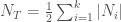
. This is the figure that is most often reported by the media. As is evident, it is impossible to determine the economic significance of this number without first knowing the structure of the market. That is, we must know how much is owed and to whom. However, after we have this information, we can choose different recovery values and then calculate each party’s exposure. This would enable us to determine how much cash each participant would have to set aside for a default at various recovery values (simply calculate each party’s exposure at the various recovery values).

Let’s consider a concrete example. In the diagram below, an edge coming from a participant represents protection sold by that participant and consequently an incoming edge represents protection bought by that participant. The amounts written beside these edges represent the notional amount of protection bought/sold. The amounts written beside the nodes represent the net notional amounts.

cds-market-diagram

In the example above, D is a dealer and his net notional amount is zero, and therefore his exposure to the risk-event is 0 \cdot M = 0 . As is evident, we can vary the recovery value to determine what each market participant’s exposure would be in that case. We could then consider other risk-events that occur in conjunction with any given risk-event. For example, we could consider the conjunctive risk-event “ABC defaults and B fails to pay under any CDS” (in which case D’s exposure would not be zero) or any other variation that addresses meaningful concerns. For now, we will focus on our single event risk for explanatory purposes. But even if we restrict ourselves to single event risks, there’s more to a CDS than just default. Collateral will move through the above system dynamically throughout the lives of the contracts. In order to understand how we can analyze the systemic risks posed by the dynamic shifting of collateral, we must first examine what it is that causes collateral to be posted under a CDS.

We’re In The Money

CDS contracts come in and out of the money to a party based on the price of protection. If a party is out of money, the typical market practice is to require that party to post collateral. For example, if I bought protection at a price of 50bp, and suddenly the price jumps to 100bp, I’m in the money and my counterparty is out of the money. Thus, my counterparty will be required to post collateral. We can view the price of protection as providing an implied probability of default. Exactly how this is done is not important. But it should be clear that there is a connection between the cost of protecting debt and the probability of default on that debt (the higher the probability the higher the cost). Thus, as the implied probability of default changes over the life of the agreement, collateral will change hands.

Collateral Flow Analysis

In the previous sections, we assumed that the risk-event was certain to occur and then calculated the exposures based on an assumed recovery value. So, in effect, we were asking “what happens when parties settle their contracts at a given recovery value?” But what if we want to consider what happens before any default actually occurs? That is, what if we want to consider “what happens if the probability of default is p?” Because collateral will be posted as the price of protection changes over the life of the agreement and the price of protection provides an implied probability of default, it follows that the answer to this question should have something to do with the flow of collateral.

Continuing with the ABC bond example above, we can examine how collateral will move through the system by asking two questions: (i) what is the implied probability of the risk-event (ABC’s default) occurring and (ii) what is the expected value of the risk-magnitude (the basis upon which collateral payments are made). As discussed above, the implied probability of default will change over the life of the agreement, which will in turn affect the flow of collateral in the system. Since our goal in this section is to test the system’s behavior at different implied probabilities of default, the expected value of our risk-magnitude should be a function of an assumed implied probability of default. So, we define the expected value of our risk-magnitude as M_e = p^* \cdot M where p^* is our assumed implied probability of default and M is defined as it is above. It follows that this analysis will break CDS contracts into categories according to the price at which they were entered into. That is, you can’t ask how much something changed without first knowing what it was to begin with.

Assume that P_i entered into CDS contracts at m_i different prices. For example, he entered into four contracts at 20 bp and eight contracts at 50bp, and no others. In this case, m_i = 2. For each P_i, assign an arbitrary ordering, (c_{i,1}, ... , c_{i,m_i}), to the sets of contracts that were entered into at different prices by P_i. In the example where m_i = 2, we could let c_{i,1} be the set of eight contracts entered into at 50bp and let c_{i,2} be the set of four contracts entered into at 20 bp. Each of these sets will have a net notional amount and an implied probability of default (since each is categorized by price). Define n_{i,j} as the net notional amount of the contracts in c_{i,j} and p_{i,j} as the implied probability of default of the contracts in c_{i,j} for each 1 \leq j \leq m_i. We define the expected exposure of
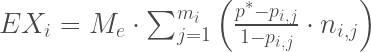
 P_i as:

EX_i = M_e \cdot \sum_{j = 1}^{m_i}\left(\frac{p^* - p_{i,j}}{1 - p_{i,j}} \cdot n_{i,j}\right) .

Note that when p^* = 1,

EX_i = M \cdot \sum_{j = 1}^{m_i}\left(\frac{1 - p_{i,j}}{1 - p_{i,j}} \cdot n_{i,j}\right) = M \cdot N_i .

That is, this is a generalized version of the settlement analysis above, and when we assume that default is certain, collateral flow analysis reduces to settlement flow analysis.

So What Does That Awful Formula Tell Us?

A participant’s expected exposure is a reasonable estimate for the amount of collateral that will be posted or received by that participant at an assumed implied probability of default. The exact amount of collateral that will be posted or received under any contract will be determined by the terms of that contract. As a result, our model is approximate and not exact. However, the direction that collateral moves in our model is exact. That is, if a party’s expected exposure is negative, it will not receive collateral, and if it is positive, it will not post collateral. It also shows that even if a party is completely hedged in the event of a default, it is possible that it is not completely hedged to posting collateral. That is, even if it bought and sold the same notional amount of protection, it could have done so at different prices.

The Mythology Of Credit Default Swaps

Systemic Speculation

Pundits from all corners have been chiming in on the debate over derivatives. And much like the discourse that has dominated the rest of human history, reason, temperance, and facts play no role in the debate. Rather, the spectacular, outrage, and irrational blame have been the big winners lately. As a consequence, credit default swaps have been singled out as particularly dangerous to the financial system. Why credit default swaps have been targeted as opposed to other derivatives is not entirely clear to me, although I do have some theories. In this article I debunk many of the common myths about credit default swaps that are circulating in the popular press. For an explanation of how credit default swaps work, see this article.

The CDS Market Is Not The Largest Thing Known To Humanity

The media likes to focus on the size of the market, reporting shocking figures like $45 trillion and $62 trillion. These figures refer to the notional amount of the contracts, and because of netting, these figures do not provide a meaningful picture of the amount of money that will actually change hands. That is, without knowing the structure of the credit default swap market, we cannot determine the economic significance of these figures. As such, these figures should not be compared to real economic indicators such as GDP.

But even if you’re too lazy to think about how netting actually operates, why would you focus on credit default swaps? Even assuming that the media’s shocking double digit trillion dollar amounts have real economic significance, the credit default swap market is not even close in scale to the interest rate swap market, which is an even more shocking $393 trillion market. But alas, we are in the midst of a “credit crisis” and not an “interest rate crisis.” As such, headlines containing the terms “interest rate swap” will not fare as well as those containing “credit default swap” in search engines or newsstands. Perhaps one day interest rate swaps will have their moment in the sun, but for now they are an even larger and equally unregulated market that’s just as boring and uneventful as the credit default swap market.

Credit Default Swaps Do Not Facilitate “Gambling”

One of the most widely stated criticisms of credit default swaps is that they are a form of gambling. Of course, this allegation is made without any attempt to define the term “gambling.” So let’s begin by defining the term “gambling.” In my mind, the purest form of gambling involves the wager of money on the outcome of events that cannot be controlled or predicted by the person making the wager. For example, I could go to a casino and place a $50 bet that if a casino employee spins a roulette wheel and spins a ball onto the wheel, the ball will stop on the number 3. In doing so, I have posted collateral that will be lost if an event (the ball stopping on the number 3) fails to occur, but will receive a multiple of my collateral if that event does indeed occur. I have no ability to affect the outcome of the event and more importantly for our purposes, I have absolutely no way of predicting what the outcome will be. In short, my “investment” is a blind guess as to the outcome of a random event.

Now let’s compare that with someone (B) buying protection on ABC’s bonds through a credit default swap. Assume that B is as villainous as he could be: that is, assume that he doesn’t own the underlying bond. This evildoer is in effect betting upon the failure of ABC. What a nasty thing to do. And why would he do such a thing? Well, B might reasonably believe that ABC is going to fail in the near future based on market conditions and information disclosed by ABC. But why should someone profit from ABC’s failure? Because if B’s belief in ABC’s impending failure is shared by others, their collective selfish desire to profit will push the price of protection on ABC’s bonds up, which will signal to the market-at-large that the CDS market believes that there will be an event of default on ABC issued debt. That is, a market full of people who specialize in recognizing financial disasters will inadvertently share their expertise with the world.

So, in the case of the roulette wheel, we have money committed to the occurrence of an event that cannot be controlled or predicted by the person making the commitment. Moreover, this “investment” is made for no bona fide economic purpose with an expected negative return on investment. In the case of B buying protection through a CDS on a bond he did not own, we have money committed to the occurrence of an event that cannot be controlled by B but can be reasonably predicted by B, and through collective action we have the serendipitous effect of sharing information. To call the latter gambling is to call all of investing gambling. For there is no difference between the latter and buying stock, buying bonds, investing in the college education of your children, etc.

The Credit Default Swap Market Is Not An Insurance Market

Credit default swaps operate like insurance at a bilateral level. That is, if you only focus on the two parties to a credit default swap, the agreement operates like insurance for both parties. But to do so is to fail to appreciate that a credit default swap is exactly that: a swap, and not insurance. Swap dealers are large players in the swap markets that buy from one party and sell to another, and pocket the difference between the prices at which they buy and sell. In the case of a CDS dealer, dealer (D) sells protection to A and then buys protection from B, and pockets the difference in the spreads between the two transactions. If either A or B has dodgy credit, D will require collateral. Thus, D’s net exposure to the bond is neutral. While this is a simplified explanation, and in reality D’s neutrality will probably be accomplished through a much more complicated set of trades, the end goal of any swap dealer is to get close to neutral and pocket the spread.

cds-swap-dealer

That said, insurance companies such as MBIA and AIG did participate in the CDS market, but they did not follow the business model of a swap dealer. Instead, they applied the traditional insurance business model to the credit default swap market, with notoriously less than stellar results. The traditional insurance business model goes like this: issue policies, estimate liabilities on those policies using historical data, pool enough capital to cover those estimated liabilities, and hopefully profit from the returns on the capital pool and the fees charged under the policies.  Thus, a traditional insurer is long on the assets it insures while a swap dealer is risk-neutral to the assets on which it is selling protection, so long as its counterparties pay. So, a swap dealer is more concerned about counterparty risk: the risk that one of its counterparties will fail to payout. As mentioned above, if either counterparty appears as if it is unable to pay, it will be required to post collateral. Additionally, as the quality of the assets on which protection is written deteriorates, more collateral will be required. Thus, even in the case of counterparty failure, collateral will mitigate losses.

This collateral feature is missing on both ends of the traditional insurance model. Better put, there is no “other end” for a traditional insurer. That is, the insurance business model does not hedge risk, it absorbs it. So if a traditional insurer sold protection on bonds that had risks it didn’t understand, e.g., mortgage backed securities, and it consequently underestimated the amount of capital it needed to store to meet liabilities, it would be in some serious trouble. A swap dealer in the same situation, even if its counterparties failed to appreciate these same risks, would be compensated gradually over the life of the agreement through collateral.

Securitization Demystified

What Is Securitization?

Securitization is a process that allows the cash flows of an asset to be isolated from the cash flows of that asset’s original owner. There are countless variations on this theme, and since our purpose here at derivative dribble is to foster clarity and simplicity, we will discuss only the main theme, and will avoid the Glen Gould variations.

Cui Bono?

We will explain how securitization works by first exploring the most basic motivation for isolating assets: access to cheaper financing. Assume B is a local bank that focuses primarily on taking deposits and earning money through very low risk investments of those deposits. Further, assume that B is a stable and solvent bank, but that it lacks the credit quality of some of the larger national banks and as such it has a higher cost of financing. This higher cost of financing means that it can’t lend at the same low rates as national banks. B’s local community is one in which home values are high and stable, and as a result the rate of default on mortgages is extremely low. As such, B would like to be able to compete in the local mortgage market, but is struggling to do so because its rates are higher than the national banks. What B would really like to do is borrow money for the limited purpose of issuing mortgages in its local community. That is, B wants to separate its credit quality from the credit quality of the mortgages it issues in its community. Securitization is the process that facilitates this isolation.

The Nuts And Bolts

The overall process is quite simple and reasonable, despite its portrayal in the popular press. We know that so long as B owns the mortgages, B’s creditors will still consider B’s credit as an institution when lending to it, even if that lending is for the limited purpose of issuing local mortgages. The solution to that problem is simple: B sells the mortgages off shortly after issuing them. But to whom? Well, common sense tells us that investors are not going to be too excited about buying mortgages piecemeal. So, B will wait until it has issued a pool of mortgages large enough to attract the attention of investors. Then, it will set up a special purpose vehicle (SPV) where that SPV’s special purpose is to buy the mortgages from B, using money from the investors, and issue notes to those same investors.

So, the SPV owns the mortgages since B is completely bought out by the cash from the investors. And the notes issued to the investors are basically bonds issued by the SPV with the mortgages as collateral. As a result, B is out of the picture from an investor’s perspective. In reality, B might still service the mortgages (i.e., sending bills to borrowers, maintaining address information on borrowers, etc.) but because the mortgages have been sold to the SPV, the notes issued by the trust have no credit risk exposure to B. So if B goes bust, the assets in the SPV are safe and will continue to pay.

So What Does That Accomplish?

B wanted to enter the local mortgage market but was struggling to do so because it couldn’t lend at the same rates as national banks. This was due to B’s inferior credit standing relative to large national banks. But the securitization process above allows B to isolate the credit quality of the mortgages it issues from its own credit quality as an institution. Thus, the rate paid on the notes issued by the SPV will be determined by examining the credit quality of the mortgages themselves, with no reference to B. Since the rate on the notes is determined only by the quality of the mortgages, the rate on any individual mortgage will be determined by the quality of that mortgage. As such, B will be able to issue mortgages to its local community at the market rate and profit from this by servicing the mortgages for a fee.

Derivatives/Synthetic Instruments Demystified

What Is A Derivative?

A derivative is a contract that derives its value by reference to “something else.” That something else can be pretty much anything that can be objectively observed and measured. For example, two parties, A and B, could get together and agree to take positions on the Dow Jones Industrial Average (DJIA). That’s an index that can be objectively observed and measured. A could agree to pay B the total percentage-wise return on that index from October 31, 2007 to October 31, 2008 multiplied by a notional amount, where that amount is to be paid on October 31, 2008. In exchange, B could agree to make quarterly payments of some percentage of the notional amount (the swap fee) over that same time frame. Let’s say the notional amount is $100 (a position that even Joe The Plumber can take on); the swap fee is 10% per annum; and the total return on the DJIA over that period is 15%. It doesn’t take Paul Erdős to realize that this leaves B in the money and A out of the money (A pays $15 and receives $10, so he loses $5).

But what if the DJIA didn’t gain 15%? What if it tanked 40% instead? In that case, we have to look to our agreement. Our agreement allocated the DJIA’s returns to B and fixed payments to A. It didn’t mention DJIA loss. The parties can agree to distribute gain and loss in the underlying reference (the DJIA) any way they like: that’s the beauty of enforceable contracts. Let’s say that under their agreement, B agreed to pay the negative returns in the DJIA multiplied by the notional amount.  If the market tanked 40%, then B would have made the fixed payments of 10% over the life of the agreement, plus another 40% at the end. That leaves him down $50. Bad year for B.

Follow The Money

So what is the net effect of that agreement? B always pays 10% to A, whether the DJIA goes up, down, or stays flat over the relevant time frame. If the DJIA goes up, A has to pay B the percentage-wise returns. If the DJIA goes down, B has to pay A the percentage-wise losses. So, A profits if the DJIA goes down, stays flat, or goes up less than 10% and B profits if the DJIA goes up more than 10%. So, A is short on the DJIA going up 10% and B is long on the DJIA going up 10%. This is accomplished without either of them taking actual ownership of any stocks in the DJIA. We say that A is synthetically shorting the DJIA and B is synthetically long on the DJIA. This type of agreement is called a total return swap (TRS). This TRS exposes A to the risk that the DJIA will appreciate by more than 10% over the life of the agreement and B to the risk that the DJIA will not appreciate by more than 10%.

What Is Risk?

There are a number of competing definitions depending on the context. My own personal view is that risk has two components: (i) the occurrence of an event and (ii) a magnitude associated with that event. This allows us to ask two questions: What is the probability of the event occurring? And if it occurs, what is the expected value of its associated magnitude? We say that P is exposed to a given risk if P expects to incur a gain/loss if the risk-event occurs. For example, in the TRS between A and B, A is exposed to the risk that the DJIA will appreciate by more than 10% over the life of agreement. That risk has two components: the event (the DJIA appreciating by more than 10%) and a magnitude associated with that event (the amount by which it exceeds 10%). In this case, the occurrence of the event and its associated magnitude are equivalent (any non-zero positive value for the magnitude implies that the event occurred) and so our two questions reduce to one question: what is the expected value of the DJIA at the end of the agreement? That obviously depends on who you ask. So, can we then infer that A expects the DJIA to gain less than 10% over the life of the agreement? No, we cannot. If A actually owns $100 worth of the DJIA, A is fully hedged and the agreement is equivalent to bona fide financing. That is, A has no exposure to the DJIA (short on the DJIA through the TRS and long through actually owning it) and makes money only through the swap fee. B’s position is the same whether A owns the underlying index or not: B is long on the DJIA, as if he actually owned it. That is, B has synthesized exposure to the DJIA. So, if A is fully hedged the TRS is equivalent to a financing agreement where A “loans” B $100 to buy $100 worth of the DJIA, and then A holds the assets for the life of agreement (like a collateralized loan). As such, B will never agree to pay a swap fee on a TRS that is higher than his cost of financing (since he can just go get a loan and buy the reference asset).

How Derivatives Create, Allocate, And “Transfer” Risk

It is commonly said that derivatives transfer risk. This is not technically true, but often appears to be the case.  Derivatives operate by creating risks that were not present before the parties entered into the derivative contract. For example, assume that A and B enter into an interest rate swap, where A agrees to pay B a fixed annual rate of 8% and B agrees to pay A a floating annual rate, say LIBOR, where each is multiplied by a notional amount of $100. Each party agrees to make quarterly payments. Assume that on the first payment date, LIBOR = 4%.  It follows that A owes B $2 and B owes A $1. So, after netting, A pays B $1.

Through the interest rate swap, A is exposed to the risk that LIBOR will fall below 8%. Similarly, B is exposed to the risk that LIBOR will increase above 8%. The derivative contract created these risks and assigned them to A and B respectively. So why do people say that derivatives transfer risk? Assume that A is a corporation and that before A entered into the swap, A issued $100 worth of bonds that pay investors LIBOR annually. By issuing these bonds, A became exposed to the risk that LIBOR would increase by any amount. Assume that the payment dates on the bonds are the same as those under the swap. A’s annual cash outflow under the swap is (.08 – LIBOR) x 100. It’s annual payments on the bonds are LIBOR x 100. So it’s total annual cash outflow under both the bonds and the swap is:

(.08 – LIBOR) x 100 +  LIBOR x 100 = .08 x 100 – LIBOR x 100  + LIBOR x 100 = 8%.

So, A has taken its floating rate LIBOR bonds and effectively transformed them into fixed rate bonds. We say that A has achieved this fixed rate synthetically.

At first glance, it appears as though A has transferred its LIBOR exposure to B through the swap.  This is not technically true. Before A entered into the swap, A was exposed to the risk that LIBOR would increase by any amount. After the swap, A is exposed to the risk that LIBOR will fall under 8%. So, even though A makes fixed payments, it is still exposed to risk: the risk that it will pay above its market rate of financing (LIBOR). For simplicity’s sake, assume that B was not exposed to any type of risk before the swap. After the swap, B is exposed to the risk that LIBOR will rise above 8%. This is not the same risk that A was exposed to before the swap (any increase in LIBOR) but it is a similar one (any increase in LIBOR above 8%).

So What Types Of Risk Can Be Allocated Using Derivatives?

Essentially any risk that has an objectively observable event and an objectively measureable associated magnitude can be assigned a financial component and allocated using a derivative contract. There are derivative markets for risks tied to weather, energy products, interest rates, currency, etc. Wherever there is a business or regulatory motivation, financial products will appear to meet the demand. What is important is to realize that all of these products can be analyzed in the same way: identify the risks, and then figure out how they are allocated. This is usally done by simply analyzing the cash flows of the derivative under different sets of assumptions (e.g., the DJIA goes up 15%).

Netting Demystified

Netting Is For Everyone, Not Just Fancy Swap Traders

Unlike most terms used in the derivatives world, netting is a good one. It has an intuitive, albeit hokey, feel (unlike other rather sterile terms such as “synthetic collateralized debt obligation”). After all, economics is about human decisions and actions, and as such, it can stand to be a bit hokey. So what is netting? The concept stems from a very simple observation: if I owe you $5 and you owe me $10, you should just give me $5. We could have several debts between the two of us, (e.g., I owe you $2 from Wednesday, $3 from Thursday), but assume we add those up into one debt per person, resulting in one transactional leg (line connecting us) each. In this case, netting would save us a bit of trouble since we only exchange money once, instead of twice.

That Is So Obvious And Trivial That It Can’t Be Right

The observation above is indeed an example of the same principle (netting) that is applied to swaps. Our example however, only has 2 parties. The time saved from engaging in 1 transaction instead of 2 is minimal, especially when it’s a transaction for such a small amount of money. This is a result of the fact that when there are only 2 parties, let’s say you and me, there are only 2 legs to the transaction: the money coming out of me and the money coming out of you. The netting example above reduces that to 1 leg (you pay me). That’s called bilateral netting. Again, when there are only 2 parties, the application of netting is simple. But the number of legs increases dramatically as we increase the number of parties (for my fellow graph theorists, the number of legs is twice the number of edges in a complete graph with N nodes, where N is the number of parties). For example,  consider the obligations of 3 friends: A, B and C. A owes B $2; A owes C $3; B owes A $4; B owes C $5; C owes A $2; and finally C owes B $6.

We apply bilateral netting to each of the pairs. That leaves us with the following: A owes C $1; B owes A $2; and C owes B $1. We could just execute 3 transactions and call it a day. But we’re smarter than that. We notice that C is basically passing the $1 from A onto B. That is, his inflow is the same as his outflow, so he serves no purpose in our transaction. So, we cut him out of the picture:

Note that the last step we just took, cutting C out, was not bilateral netting. It was a different kind of netting. It required a different observation, but the principle is the same: only engage in necessary transactions. Finally, we apply bilateral netting to the transaction between A and B. So, in the end, that complex sea of relationships boiled down to B paying A $1.

Balsamic Reduction

Rather then execute a disastrously complicated web of transactions, swap dealers, and ordinary banks, use clearing houses to do exactly what we just did above, but on a gigantic scale. Obviously, this is done by an algorithm, and not by hand. Banks, and swap dealers, prefer to strip down the number of transactions so that they only part with their cash when absolutely necessary. There are all kinds of things that can go wrong while your money spins around the globe, and banks and swap dealers would prefer, quite reasonably, to minimize those risks.

An Engine Of Misunderstanding

As you can see from the transactions above, the total amount of outstanding debts is completely meaningless. That complex web of relationships between A, B, and C, reduced to 1 transaction worth $1. Yet, the media would have certainly reported a cataclysmic 2 + 3 + 4 + 5 + 2 + 6 = $22 in total debts.

Systemic Counterparty Confusion: Credit Default Swaps Demystified

It Is A Tale Told By An Idiot

The press loves a spectacle. There’s a good reason for this: panic increases paranoia, which increases the desire for information, which increases their advertising revenues. Thus, the press has an incentive to exaggerate the importance of the events they report. As such, we shouldn’t be surprised to find the press amping up fears about the next threat to the “real economy.”

When written about in the popular press, terms such as “derivative” and “mortgage backed security” are almost always preceded by adjectives such as “arcane” and “complex.” They’re neither arcane nor complex. They’re common and straightforward. And the press shouldn’t assume that their readers are too dull to at least grasp how these instruments are structured and used. This is especially true of credit default swaps.

Much Ado About Nothing

So what is the big deal about these credit default swaps? Surely, there must be something terrifying and new about them that justifies all this media attention? Actually, there really isn’t. That said, all derivatives allow risk to be magnified (which I plan to discuss in a separate article). But risk magnification isn’t particular to credit default swaps. In fact, considering the sheer volume of spectacular defaults over the last year, the CDS market has done a damn good job of coping.  Despite wild speculation of impending calamity by the press, the end results have been a yawn . So how is it that Reuters went from initially reporting a sensational $365 billion in losses to reporting (12 days later) only $5.2 billion in actual payments? There’s a very simple explanation: netting, and the fact that they just don’t understand it. The CDS market is a swap market, and as such, the big players in that market aren’t interested in taking positions where their capital is at risk. They are interested in making money by creating a market for swaps and pocketing the difference between the prices at which they buy and sell. They are classic middlemen and essentially run an auction house.

Deus Ex Machina

The agreements that document credit default swaps are complex, and in fairness to the press, these are not things we learn about in grammar school – for a more detailed treatment of these agreements, look here. Despite this, the basic mechanics of a credit default swap are easy to grasp. Let’s begin by introducing everyone: protection buyer (B) is one party and swap dealer (D) is the other. These two are called swap counterparties or just counterparties for short. Let’s first explain what they agree to under a credit default swap, and then afterward, we’ll examine why they would agree to it.

What Did You Just Agree To?

Under a typical CDS, the protection buyer, B, agrees to make regular payments (let’s say monthly) to the protection seller, D. The amount of the monthly payments, called the swap fee, will be a percentage of the notional amount of their agreement. The term notional amount is simply a label for an amount agreed upon by the parties, the significance of which will become clear as we move on. So what does B get in return for his generosity? That depends on the type of CDS, but for now we will assume that we are dealing with what is called physical delivery. Under physical delivery, if the reference entity defaults, D agrees to (i) accept delivery of certain bonds issued by the reference entity named in the CDS and (ii) pay the notional amount in cash to B. After a default, the agreement terminates and no one makes anymore payments. If default never occurs, the agreement terminates on some scheduled date. The reference entity could be any entity that has debt obligations.

Now let’s fill in some concrete facts to make things less abstract. Let’s assume the reference entity is ABC. And let’s assume that the notional amount is $100 million and that the swap fee is at a rate of 6% per annum, or $500,000 per month. Finally, assume that B and D executed their agreement on January 1, 2008 and that B made its first payment on that day.  When February 1, 2008 rolls along, B will make another $500,000 payment. This will go on and on for the life of the agreement, unless ABC triggers a default under the CDS. Again, the agreements are complex and there are a myriad of ways to trigger a default. We consider the most basic scenario in which a default occurs: ABC fails to make a payment on one of its bonds. If that happens, we switch into D’s obligations under the CDS. As mentioned above, D has to accept delivery of certain bonds issued by ABC (exactly which bonds are acceptable will be determined by the agreement) and in exchange D must pay B $100 million.

Why Would You Do Such A Thing?

To answer that, we must first observe that there are two possibilities for B’s state of affairs before ABC’s default: he either (i) owned ABC issued bonds or (ii) he did not. I know, very Zen. Let’s assume that B owned $100 million worth of ABC’s bonds. If ABC defaults, B gives D his bonds and receives his $100 million in principal (the notional amount). If ABC doesn’t default, B pays $500,000 per month over the life of the agreement and collects his $100 million in principal from the bonds when the bonds mature. So in either case, B gets his principal. As a result, he has fully hedged his principal. So, for anyone who owns the underlying bond, a CDS will allow them to protect the principal on that bond in exchange for sacrificing some of the yield on that bond.

Now let’s assume that B didn’t own the bond. If ABC defaults, B has to go out and buy $100 million par value of ABC bonds. Because ABC just defaulted, that’s going to cost a lot less than $100 million. Let’s say it costs B $50 million to buy ABC issued bonds with a par value of $100 million. B is going to deliver these bonds to D and receive $100 million. That leaves B with a profit of $50 million. Outstanding. But what if ABC doesn’t default? In that case, B has to pay out $500,000 per month for the life of the agreement and receives nothing. So, a CDS allows someone who doesn’t own the underlying bond to short the bond. This is called synthetically shorting the bond. Why? Because it sounds awesome.

So why would D enter into a CDS? Again, most of the big protection sellers buy and sell protection and pocket the difference. But, this doesn’t have to be the case. D could sell protection without entering into an offsetting transaction. In that case, he has synthetically gone long on the bond. That is, he has almost the same cash flows as someone who owns the bond.

The Not So Efficient Market (Theorem) Hypothesis

Are Capital Markets Efficient?

Let’s examine the question using elementary game theory. That is, let’s assume that given any decision, each capital market participant acts in a way that maximizes his expected utility.

But How Would We Do That?

First we explore one example of incentive structures which leads to a sell off. Then we consider how the Efficient Market Hypothesis fits into the framework of economic knowledge and the notion of economic efficiency. Finally, we conclude that even if a capital market incorporates all available price-information, it is possible that the outcome is not an efficient allocation of capital.

The Sound And The Fury

Assume that Apocalypse Ann (A) and Tag Along Teds (T1, T2, …, Tn) are all traders that hold large positions in ABC stock. Assume that A is convinced that ABC is doomed because of recent conditions in the credit markets. She may or may not be correct in her prediction, but assume she honestly believes that ABC will be placed into receivership and liquidated, with little to no money left for equity holders.  Further, assume that each of T1, T2, …, Tn is aware of A’s belief. Personally, each thinks that A is out of her mind, that ABC is well positioned to ride the current credit crisis and that current equity valuations of ABC are rational. However, they know that given A’s belief, she will certainly liquidate her position.

Assume that each of T1, T2, …, Tn is a trader for a fund that has some rather jittery investors who are awaiting quarterly results and approaching a point in their investments where they have the right to withdraw their investment.  Assume that L is the maximum decrease in total value of any ABC position that any investor in any of the funds will accept for the quarter without withdrawing their investment; and assume that no trader wants its investors to withdraw.

Assume that based on historical data and current trading volumes, if the current price of ABC stock is P1, then the price after A liquidates a 100 share lot is expected to be P2 = Δ × P1, for some  0 < Δ ≤ 1. Let the number of shares held by A be k × 100; let S be the smallest number of ABC shares held by any one of  T1, T2, …, Tn; and let P be the current price of ABC’s stock.  For any Δ < 1, we can choose k such that L < S \times P \times (1 - \Delta ^{k} ) . That is, the expected decrease in the smallest position of ABC’s stock held by any of T1, T2, …, Tn as a result of A liquidating her position is greater than the maximum decrease in total value that any investor will accept without withdrawing their investment. Therefore, each of T1, T2, …, Tn will try to sell their positions before A does so, further deteriorating the price of ABC stock. Moreover, each has an incentive to be the first to sell.

Interesting, But That Looks Like A Very Specific Scenario

While catered to fit our current economic context, the root of the problem comes from the interactions between two sets of facts: the group of investors (the Teds) with a contingent investment horizon that could shorten dramatically upon the occurrence of a particular event (if the price of ABC tanks, the Teds’ investment horizons collapse to the present because the investors will want their money back); and the fact that the occurrence of that event is in the control of another party that benefits (or at least believes they will benefit) from its occurrence.

In the example, Ann acts as an individual. In theory and reality, Ann could be an individual or a group of individuals. Ann could be a group of short sellers. Ann could be a large bank that was forced to liquidate its assets. It doesn’t matter. So long as Ann will certainly liquidate a sufficiently large enough position, the Teds will as well.

But Doesn’t The EMH Imply That ABC’s Price Would Go Back Up?

EMH proponents would argue that in the case of such a mass liquidation, white knights will run in and bid the price up again if the underlying equity were truly “worth it.” This must be true on some level, since the number of sales must always equal the number of purchases. However, prices move. And “sell offs” cause prices to fall. This fact cuts to the nature of prices and is beyond the scope of this essay. We simply note that the fire sale dynamic creates its own little race to the bottom: each Ted has an incentive to lower their asking prices given the possibility that another Ted will go even lower.  Thus, the Teds are playing a game where expected utility decreases the longer it takes for them to close a sale. This entire fiasco is a result of the incorporation of relevant price information. That is, the fact that Ann will liquidate is relevant price information, and is therefore incorporated into the Teds’ decision to liquidate.

Straighten Out Your Mind’s Eye

We need to get our epistemology straight before we examine the consequences of what I’ve just outlined. First, the Efficient Market Hypothesis (EMH) is just that, a hypothesis. While there are 3 different flavors, the general idea is that all available information is quickly incorporated into the price of a stock in the world’s most developed stock markets. This hypothesis was then tested with empirical research. Whatever your opinion on how well the research actually tested that hypothesis, just assume for our purposes that the research conducted to date did test the hypothesis, and failed to prove it false.

Even if we assume that the EMH is supported by empirical evidence, its name is still a misnomer. While it does assume that information is observed and then quickly incorporated into the price of a stock, that process does not fit nicely into any well accepted notion of efficiency. For the EMH does not treat information as a good to be efficiently allocated. It boldly assumes that information is automatically available and incorporated to the maximum extent: to the point where no one could create an opportunity for arbitrage through the use of any information. This assumption is in and of itself puzzling and undermines the notion that information has value, which it clearly does. So, I prefer to think of pricing, which includes the incorporation of available price-information, as anterior to efficiency. That is, if assets are accurately priced, then resources will be allocated efficiently among those assets. This allows us to separate the EMH itself (the informational aspect) from its implications (efficiency). So, the EMH implies that the equity prices of companies trading in the most advanced capital markets will accurately reflect all available information, and that therefore capital will be distributed efficiently within those markets.

So How Is That Inefficient?

Good Question. As discussed earlier, the main purpose of assuming the EMH is true is to convince us that the markets distribute capital efficiently. (The observation and incorporation of information is itself interesting and important, but the goal is to allocate goods based on that information). While there are competing definitions of efficiency, the general gist is that a market is said to distribute capital efficiently if there’s no better way to distribute capital than the distribution created by the market: there might be other distributions that are just as good, but no distribution is better. “Good” and “better” are clearly imprecise terms, and we should have some definition of utility that we seek to maximize in the capital markets. However, the outcome of the Ann and Ted scenario is sub optimal under any reasonable definition of utility.

The purpose of the capital markets is to distribute capital to companies. The EMH takes as one of its corollaries that this distribution is efficient. However, as demonstrated above, the separation of control over an event and contingent investment horizons keyed to that event can lead to changes in equity prices that have nothing to do with the financial health of the underlying company. The result is that a company that becomes subject to such a situation will have a higher of cost raising capital through equity.

Q.E.D.

Assume that the state of affairs before the ABC sell off was efficient. We assume that when all other variables are fixed, there is only one efficient cost of equity capital for any company. Therefore, all variables other than the sell off being fixed, because ABC’s cost of equity capital has deviated from an efficient level, the state of affairs after the sell off must be inefficient. So, something else must have changed if the state of affairs after the sell off is to be efficient. In theory, this is entirely possible. In reality, however, given that panic sales usually go to cash or cash equivalents, it is not likely. Thus, theory agrees with common sense: even if the EMH is true, panic sales are still possible and lead to inefficient results. That is, whether or not the timely observation and incorporation of relevant price-information is a necessary condition for efficient allocation of capital, it is not a sufficient condition.