Update on Norwegian Ancestry

July 19, 2024July 20, 2024 / erdosfan / Leave a comment

I wrote a note a while back on Norwegian ancestry [1], and in that note I show that about 14% of Norwegians have Thai mtDNA, whereas about 6% of Swedes have Thai mtDNA. The match threshold is in this case set to 99% of the full mtDNA genome, so this is not something that can be dismissed. Further, the Finns are even closer to the Thai, with about 18% of Finns again a 99% match to Thai mtDNA. Sweden is in the middle of Norway and Finland, so it’s a bit strange, since you can’t argue an East to West migration, unless the Swedes killed a lot of people that are related to the Thai, or simply didn’t reproduce with them.

I think instead we can make sense of all of this, by looking to the Sami, who are yet again even closer to the Thai, with about 30% of the Sami a 99% match to the Thai. The Sami are nomadic people that certainly extend further East than the Scandinavians, into Russia, and I think they are ultimately Asian people. If true, this would explain why the Finns are so close to the Thai, and then all you need is for the Swedes to generally avoid mating with the Finns, which is what sovereign boundaries generally accomplish. The fact that the Finns and Sami speak a totally different, Uralic language, whereas the Swedes and Norwegians speak Germanic languages, is consistent with this hypothesis.

This still leaves the question of why the Norwegians are so close to the Thai. I previously noted in [1] that Norway, and not Sweden, has a large number of churches, that are plainly Asian in design, and Thai in particular. Below is (1 left) the distribution of Stave Churches, none of which are in Sweden, though they are elsewhere in Europe, (2 center) the Borgund Stave Church, and (3 right) the Sanctuary of Truth in Thailand.

The question is, why were these churches (all built around 800 years ago) only built in Norway, and not Sweden, and further, how on Earth did Thai mtDNA end up in Norway in such a large quantity?

I think the answer is actually quite simple: Nordic people travelled to Thailand, which is consistent with the fact that the Vikings had Buddhist relics. Further, I can’t find a single Viking monument that is still standing, other than the Runic Stones, basically all of which are in Sweden. I think Nordic people, presumably the Vikings, travelled to what is now Thailand, and learned how to construct buildings that last, out of wood. This might sound backwards from the basically racist modern perspective, but the Khmer Empire e.g., constructed massive temples that are still standing to this day, and had very advanced skills in the fine arts generally. Below is (1 left) Angkor Wat and (2 right) is a bust of Jayavarman VII, both of which are plainly superior in quality to anything produced by the Vikings, by a simply enormous margin, except the Viking ships. Both of these were again produced about 800 years ago, the same age as the Stave Churches.

Despite having drastically superior building and artisan skills generally, it seems at least credible that the people of South East Asia, around the time of the Khmer Empire, didn’t have the best ships. That AP article says that the Khmer Empire ship in question was cut from a single tree trunk. That is nothing compared to the ships constructed by the Vikings, which were at their extremes, almost three times as large, and extremely complex structures. Below is (1 left) the Oseburg ship, built around 1,200 years ago, (2 right) a detail from the Oseburg ship, and (3 right) a detail from the Urnes Stave Church, which is plainly similar to the detail from the Oseburg ship (and neither look terribly Christian to me).

Again, the Khmer ship is from almost exactly the time these Stave Churches are believed to have been built, about 800 years ago. This suggests the possibility that a bargain was struck, where a people that knew how to construct large, durable buildings (i.e., the South East Asians), exchanged that knowledge, for the ability to build large durable ships, or simply bought them from the Nordic people. A really interesting possibility is that this led to the settlement of Hawaii, which would obviously require seriously advanced navigation skills. Hawaii was believed to be settled around the same time, roughly 800 years ago, but this is still not totally sorted (to my limited knowledge on the topic). If you look through my work on mtDNA generally, you’ll see that about 50% of the Thai are a 99% match to the Hawaiians, making this a not totally ridiculous hypothesis.

The bottom line is, the Vikings probably didn’t know how to construct large durable buildings, until either someone figured it out, or someone else taught them. At the same time, if this is true, they sailed all the way to South East Asia, which is an astonishing accomplishment. In the case of the Khmer, it seems plausible that what was plainly an incredibly advanced civilization, was still making use of primitive boats.

All of this cuts again the false notion of generalized skill, and advancement, that probably comes from the Renaissance, and was reinforced in modernity, where one country is simply “more advanced” than another. In contrast, it seems plausible that people traded in ideas, a very long time ago, becoming skilled at only particular things, and learning other skills over time from other civilizations, creating a much more complex portrait of what I suppose would be a balance of trade. This would be an early market for intellectual property, that of course makes sense, it’s just not typically expressed in these terms, because it’s history and not economics, but in this view, history is economics.

All that said, the Thai are not the Khmer, but it’s pretty close. Further, the fact that the Nordic peoples went from building (as far as I can find) literally nothing that is still standing, to building plainly Asian structures that are still standing, suggests some kind of technology transfer. My best guess is that in exchange for knowledge, or perhaps simply ships, the Nordic peoples learned about real architecture from people that lived around what is now Thailand and Cambodia, and kept the style. Now, if you did all of this, you probably wouldn’t want to share any of it, especially if you brought back women, men being who they are, in particular Viking men. This would make it perfectly sensible to seek a separate piece of land, and start what I think was a distinct Nordic culture, that eventually came to be what we know as Norway.

Knowledge and Utility

July 6, 2024July 6, 2024 / erdosfan / Leave a comment

I wrote a paper a while back called “Information, Knowledge, and Uncertainty” [1], that presents a mathematical theory of epistemology. I go on to apply it, showing that it can be used in machine learning to drastically improve the accuracy of predictions, using a measure of confidence that follows from the definitions in [1]. In some other research note that I don’t remember the name of, I pointed out that we can also think about a different kind of information that is conveyed through a proof. Specifically, that longer proofs correspond to more computational work, i.e., the work required to prove the theorem, which will have some number of deductive steps. Simply count the steps, the more steps there are, the more work required to prove the result. Now of course, you could have a “bad” and pointlessly long proof for a theorem. Simply posit the existence of a shortest proof, as an analog to the Kolmogorov Complexity. The number of steps in the shortest proof for a theorem is the depth of the theorem.

What caught my attention this morning is the potential connection between utility and the depth of a theorem. For example, the Pythagorean Theorem has very short proofs, and as a result, the shortest proof will necessarily also be short. Despite this, the Pythagorean Theorem is remarkably useful, and has undoubtedly been used relentlessly in architecture, art, and probably plenty of other areas of application. Now you could argue that there is no connection between depth and utility, but perhaps there is. And the reason I think there might be, is because I show that in [1], the more Knowledge you have in a dataset, the more accurate the predictions are, implying utility is a function of Knowledge, which has units of bits.

You can view the number of steps in a proof as computational work, which has units of changes in bits, which is different than bits, but plainly a form information. So the question becomes, is this something universal, in that when information is appropriately measured, that utility becomes a function of information? If this is true, then results like the Graph Minor Theorem and the Four Color Theorem could have profound utility, since these theorems are monstrously deep results. If you’re a cartographer or someone that designs flags, then the Four Color Theorem is already useful, but jokes aside, the point is, at least the potential, for profound utilization of what are currently only theoretical results.

As a self-congratulatory example, I proved a mathematical equivalence between sorting a list of real numbers and the Nearest Neighbor method [2]. The proof is about one page, and I don’t think you can get much shorter than what’s there. But, the point is, in the context of this note, that the utility is unreal, in that machine learning is reduced to sorting a list of numbers (there’s another paper that proves Nearest Neighbor can produce perfect accuracy).

I went on to demonstrate empirically that the necessarily true mathematical results work, in the “Massive” edition of my AutoML software BlackTree AutoML. The results are literally a joke, with my software comically outperforming Neural Networks by an insurmountable margin, with Neural Networks taking over an hour to solve problems solved in less than one second (on a consumer device) using BlackTree, with basically the same accuracy in general. Obviously, this is going to have a big impact on the world, but the real point is, what do the applications of something like the Graph Minor Theorem even look like? I have no idea. There’s another theorem in [2] regarding the maximization of some entropy-like function over vectors, and I have no idea what it means, but it’s true. I’ve dabbled with its applications, and it looks like some kind of thermodynamics thing, but I don’t know, and this is disturbing. Because again, if true, it implies that the bulk of human accomplishment has yet to occur, and it might not ever occur because our leaders are a bunch of maggots, but, if we survive, then I think the vast majority of what’s possible is yet to come.

All of that said, I’m certainly not the first person to notice that mathematics often runs ahead of e.g., physics, but I’m pretty sure I’m the first person to notice the connection (if it exists) between information and utility, at least in a somewhat formal manner. If this is real, then humanity has only scratched the surface of the applications of mathematics to reality itself, plainly beyond physics.

The Asymmetry Between Gains and Losses

June 6, 2024July 12, 2024 / erdosfan / Leave a comment

It dawned on me a while back that there’s a fundamental asymmetry between financial gains and losses, in that gains are strictly positive events from a utility or other subjective preference perspective, whereas losses are strictly negative events, but with the possibility to cause catastrophic knock-on events. Specifically, gains will never cause a default, whereas a loss can. That is, if someone gives you money, or your net worth appreciates for some other reason, this simply cannot cause a default. In contrast, if someone steals your money, or your net worth otherwise decreases for some other reason, you could default on existing liabilities, which will create not only losses for others, but potentially catastrophic financial consequences on an individual level (e.g., homelessness or even death in the case of losing health insurance). This implies that we should seek to avoid defaults as a society, as opposed to losses, which are not innately harmful to others, and not generally catastrophic to individuals (e.g., just because you lose some money in the market doesn’t mean you’ll lose your home).

The problem is that default risks are idiosyncratic, in that one firm could be perfectly fine incurring a million dollars in losses over some period of time, whereas another would go bankrupt. This means that the market for hedging loss of income (which doesn’t to my knowledge exist yet) is going to be heterogeneous, and probably not exchange traded. But so what, so is lending, and that’s nothing new to banks.

In fact, you can posit a simple market that is basically unfinanced credit exposure, where firm A buys protection on some level of income for a fixed period of time, from bank B. Specifically, firm A pays bank B to underwrite the risk that a particular asset ends up generating less than a particular amount of revenue over a particular amount of time. For example, imagine a large food chain buys such a contract from a bank, so that if one of their franchises fails to produce at least $1,000,000 in revenue per year, for a window of let’s say 5 years, the bank writes them a check for $1,000,000 – X, where X is the revenue actually generated in the year the shortfall occurred. The bank would charge a fee based upon the revenue history of the particular franchise, which is distinct from (but of course related to) the credit risk of the franchise. In fact, the whole point of this, is for the franchise itself to avoid contributing to an overall default by the food chain. I would call it a revenue shortfall swap.

This is potentially a really attractive product from the perspective of the bank, because they can contract with the food chain holding company, presumably a much better credit than the specific franchise location. As a result, the bank gets a corporate quality credit (as a counterparty), but the exposure is to a potentially highly diversified set of revenue streams, across huge, and individually selected geographies, with different consumer profiles. This should be attractive to the corporates as well, because they can micromanage revenue risk, over specific periods of time, where they might be willing e.g., to forgo some profit, in exchange for stability.

In thinking further about this, I think it could set the stage for individual employment insurance, something this country (the U.S.) desperately needs. Specifically, banks can probably use in-house municipal bond experts that have knowledge of state and local economies. This would allow them to at least contribute to the knowledge necessary to create the corporate products above, but also potentially create a market where people can buy insurance on their income (e.g., get fired, get a payout for one year equal to your previous income). This will probably be too expensive for most low income people, and frankly, banks won’t write those contracts because they’re probably bad credits, and also they won’t trust poor people to maintain employment. As a fix, I think we could instead require everyone in e.g., New York to buy employment insurance, unless you have one year in after-tax savings. This would be paid for by the state, and the high income earners (including seriously high earners that in this state make $10 million and $100 million per year), would also have to participate, unless they again have one year’s worth of after-tax cash. So e.g., Jamie Dimon would not pay into this system today, because he’s worth over a $1 billion, and makes about $40 million per year. However, a young Jamie Dimon would have to pay in, until his savings reached the one year after-tax threshold. That kind of revenue, will attract banks, and might even be enough revenue to pay for the system (people like that generally don’t get fired, and banks know this, in particular J.P. Morgan).

Bilateral Comparison of Ancestry Flows

May 30, 2024 / erdosfan / Leave a comment

In a previous note, I presented an algorithm that allows you to test ancestry flows between three populations. The method in the previous note already allows for bilateral comparisons, between the three populations. However, if you repeatedly apply the trilateral test, using all possible triplets from a dataset of populations, you will produce a graph. This graph will have bilateral flows using information derived from the entire dataset, as opposed to just three populations.

I’m still mulling through the data, but in the previous note, I stated that Norway seems to be the root population for basically everyone. I now think it’s somewhere around Holland and Denmark, using the full graph produced by the algorithm below. This is not to undermine the hypothesis that human life began in Africa, instead, the hypothesis is that modern homosapiens seem to have emerged pretty recently, in Northern Europe. All of this stuff needs to be squared off with other known results, in particular archeological results, but it does explain how, e.g., South East Asians have the gene for light skin, by descendancy (i.e., they’re the ancestors of white Europeans). I’m merely expanding the claim, pointing out that a lot of Africans also test as the descendants of Europeans, using mtDNA.

Here’s the code, more to come. You just call it from the command line saying “graph_matrix = generate_full_ancestry_graph(dataset, num_classes, N);”. The resultant graph flows are stored in graph_matrix. You’ll need the rest of the code, which is included in the paper I link to in the previous note.

generate_full_ancestry_graph Download

generate_ancestry_graph Download

Determining Ancestral Flow Across Populations

May 18, 2024October 4, 2024 / erdosfan / Leave a comment

In my paper, “A New Model of Computational Genomics” [1], I introduced an algorithm that allows you to test whether genome A is the ancestor of genomes B and C. You can read [1] to understand how it works, but for intuition, if both B and C begin identical to A, and then evolve independently in different environments, the number of bases they have in common going forward has to be the result of chance. Therefore, the genomes A and B, and A and C, should have more bases in common than B and C (i.e., both B and C deviate away from A independently of each other).

If we apply this test to three populations of genomes, instead of a single genome, we can count how many times the population A satisfied the inequality above, over all combinations of genomes selected from populations A, B, and C. Every time it is satisfied, we increment a counter associated with population A. We can then treat B and C as the ancestor (of course separately), again counting how many times the inequality is satisfied, producing a total of three counters. This will allow us to compare A, B, and C, and select the population that produced the greatest number of satisfied tests as the most likely to be the ancestor of the three populations. This is exactly what I did yesterday.

Each of the populations will again be associated with a counter that tells you how many times the inequality above is satisfied. If we divide by the total number of comparisons (i.e., the number of times we tested the inequality), we can produce a percentage. If e.g., we assume that Norway is the ancestor of Nigeria and Ancient Egypt, it turns out that test is satisfied 39.722% of the time. We can represent this as a graph with three vertices, one for each population, and a labelled edge running from the purported ancestor population to the two dependent populations. This is crudely represented below in my diagram, with an edge from Norway to both Nigeria and Ancient Egypt, labelled with the percentage of successful ancestry tests.

If we run the same tests again, this time treating each of Nigeria and Ancient Egypt as the ancestor population, we will produce an additional four edges, together producing a complete di-graph on three vertices in the form below. I nixed the labels for clarity, but did however include a new label “f”, representing the net percentage, and therefore net flow between the populations. This is easy to calculate, you just take the difference between e.g., the edge connecting A to B, and the edge connecting B to A, producing a single net figure from A to B. If the figure is positive, it means that A is more likely to be the ancestor of B, and if negative, that B is more likely to be the ancestor of A.

Below is some code that calculates the net flows for three populations, but I haven’t written any graph software yet (hence the “artwork” above). Astonishingly, Norway seems to be the root population for Nigeria and Ancient Egyptian. Now, this is subject to falsification, and there could be some other triplet of genomes that implies otherwise. That said, preliminary testing so far suggests that Northern Europeans, in particular Norwegians and Swedes, really might be the source population for a simply enormous number of people. And again, this could explain why South East Asians are literally white, genetically, which makes no sense, because it’s an extremely hot climate.

Interpreting the output below, we see that, in the context of the three populations, Norway is the best-fit ancestor of the Nigerians and Ancient Egyptians, and the Nigerians fit as a descendant of the Ancient Egyptians. What’s amazing about this, is you can use mtDNA, and literally impute geographic, directional flow, in this case, pointing mostly south, from Norway to West Africa and North East Africa. Thinking through all of this, it’s astonishing, because it’s just mtDNA, but you can literally project this onto a map, and determine geographic flows among populations.

This sounds crazy, Ancient Egyptians, they’re African! Sure, geographically, but when you look at their mtDNA, they appear to be South East Asian, and when you look at their artwork prior to Ancient Rome, they also look South East Asian. One sensible explanation, is that after the last Ice Age, about 10,000 years ago, populations that were otherwise stuck in Scandinavia started migrating. They don’t have to conquer to spread, they just have to survive with a higher probability than other populations. Given that they likely lived through Hell in a frozen tundra, once conditions improved, I think it’s perfectly sensible to assume that they survived with a higher probability than many other populations. This would cause them to spread without conquest, which seems to be the case, and I think what happened is, they ended up in South East Asia, migrating by foot (note Norwegians also test as the ancestor of Mongolians, Chinese, and Indian people, consistent with this hypothesis). Then, I think a group of South East Asians came back to the Middle East and North Africa (specifically the Pre-Roman Egyptians) by boat, which kicked off the ferocious competition of the Classical World. This is also consistent with the fact that the modern day Sri Lankans and Phoenicians are literally identical on the maternal line. This makes no sense, in the absence of interactions between the Classical World (or prior) and Asia. Also, there are obviously Asian Churches in Norway and several Buddha statues found at Viking sites. I don’t know for sure, because I’m only looking at mtDNA, but common sense suggests it’s something like this, otherwise you don’t have white people in a tropical climate like Thailand. I’ve been there, and I got horrible sunburn, it doesn’t make sense, absent an explanation like this.

Here’s the code, the dataset and any missing code can be found in [1].

net-flow-code Download

Testing Ancestry Algorithmically

May 17, 2024May 17, 2024 / erdosfan / Leave a comment

In my paper, “A New Model of Computational Genomics” [1], I presented an algorithm that allows you to test for ancestry given three genomes A, B, and C. In short, if genomes B and C descend from genome A, then genomes A and B, and genomes A and C, should have more bases in common than genomes B and C. You can read [1] to see why, but it’s mathematically impossible for B and C to have anything meaningfully more than chance in common with each other, since they both start the same (i.e., identical to genome A), and then evolve independently.

In [1], I provide the code to implement this algorithm, but tonight I wrote a really fun algorithm that finds the best root population among entire populations A, B, and C. That is, it tests, genome by genome, whether a given combination of three genomes from populations A, B, and C (one from each population), satisfies the test stated above. By doing this repeatedly, it can report back the root population with the highest percentage of satisfied tests.

I’ve noted in the past (including in [1]) that it’s obvious the Northern Europeans are closely related to the Ancient Egyptians. Specifically, it looks like they descend from the Ancient Egyptians. More recently, I’ve noticed that a lot of people globally are related to Northern Europeans. Applying the algorithm I wrote tonight, it looks like the flow is from West to East, in that e.g., when you ask whether South Koreans are the ancestors of the Norwegians and Germans, you get a low metric. In contrast, when you ask whether the Norwegians are the ancestors of the South Koreans and Germans you get a significantly higher metric. This requires a lot more testing, but it could explain why e.g., South East Asians are literally white, in the genetic sense.

Overall, my view now is that human life began in Africa, at some point turning into Denisovans, which in turn produced Neanderthals, which in turn produced modern humans. Heidelbergensis also seems to flow from Denisovans, but Heidelbergensis does not seem to be the ancestor of modern humans. You can test all of this using the code below. Really interesting, the people of Cameroon are significantly Denisovan (and so are the Finns, Danes, and Jews). In some cases, the people of Cameroon test as the ancestors of Asian Denisovans found in a cave, dated to about 50,000 years ago. This suggests at least the possibility that the people of Cameroon are the real thing, our closest link to our original ancestors, that began in Africa, moved to Asia, moved back to Africa and Europe (in particular Ancient Egypt), and then spread all over the world, including back to Asia, and South East Asia in particular. I suppose by the time they made that last journey to South East Asia, they were already white. It’s a crazy story, and it’s simply incredible that mathematics allows you to deduce all of this from just mtDNA. Note that it’s an ordinal test only, so you can’t say how long these transitions took, but you can say that one genome is the ancestor of two others.

Here’s the code, enjoy! Any missing code (and the dataset) can be found in [1].

ancestry-test Download

Using Software to Assist Speech Impediments

April 3, 2024April 3, 2024 / erdosfan / Leave a comment

It just dawned on me using my Apple Watch that you could use a simple tweak to improve dictation software, probably really easily. You just create a dataset targeted at people that have speech impediments, probably broken out by type (e.g., a lisp versus a stammer), where the training dataset is generated by people correcting text generated by the existing dictation software. That is, you use whatever dictation software you have, and then build a new dataset mapping inputs to corrected outputs. I wouldn’t even call this machine learning, it’s just a simple added layer that accounts for the fact the user has a speech impediment. In fact, you should probably allow this to be a feature in any dictation device, since someone could just have a funny voice that doesn’t map well to the training dataset or more generally, simply doesn’t perform well for whatever reason. This is a trivial adjustment, that could have real utility.

I did a quick Google search, and it looks like a simple version of this product does not exist, and instead people are using Machine Learning. There’s no way this is a hard problem, especially using machine learning. A lot of people stutter, and so there should be demand for exactly this software. I don’t have time to implement this (in particular because it requires people to generate the dataset), so you can keep this one, there it is, public domain.

On Selection and Intelligence

March 16, 2024March 16, 2024 / erdosfan / Leave a comment

Intuitively, it makes sense that intelligence would persist in Nature, because for all animals, brain power is useful and therefore at a minimum shouldn’t hurt a species. That said, it’s not clear why in particular homosapiens have grown more intelligent over time. As a general matter, selection should explain it. For example, it’s generally accepted that some kind of apocalyptic event lead to the demise of the largest dinosaurs, presumably an asteroid hitting the Earth. This killed off the largest animals above ground, presumably because they needed more food to survive than the small ones, and a catastrophic event could of course limit the total amount of food available for all animals. Smaller animals could survive on less food, and then eventually get bigger once conditions improved, which seems to be roughly what happened. So we can plainly see the mechanics involved: the total food supply literally shrinks, which kills anything that needs too much food, and whether or not this is exactly what happened, it makes sense, mechanically. Now why on Earth would animals get more intelligent as a function of time?

I think the answer is the same: disaster. When disaster strikes, the ability to predict the behavior of your environment could mean the difference between life and death. Because reality is governed by physics and mathematics, disaster could again be responsible for the selection of intelligence. So it’s indirect in this view: disaster forces selection for mechanical intuition and mathematics, and both of those require intelligence. Just imagine starting a fire near a bunch of wolves, near a body of water. Now set that same fire near a bunch of monkeys. Do the same with a bunch of people. Only the stupidest people won’t realize that the water probably won’t set on fire, whereas the same is not true of the wolves, and might not be true of the monkeys. That’s all you need to have literally all animals replaced by humans, disaster, and further, that’s all you need to get rid of stupid people as well, which could explain why humans have generally become more intelligent as a function of time.

Keep in mind a UTM is equivalent to processing language, suggesting that once you speak a language, you have all the intelligence you need, as a technical matter, to do all of computable mathematics. This suggests that in some sense humanity peaked at the development of language, and I think this could explain the proliferation of Phoenician-like languages, all the way out to Mongolia, for the simple reason that the Phoenicians might have been the first people to develop a written language, of course taking into account the possibility of a prior group that was subject to disaster.

On the Complexity of a Graph

March 16, 2024May 23, 2024 / erdosfan / Leave a comment

Introduction

I’ve been thinking about representational complexity for a long time, and in fact one of the first papers I wrote was on the intersection number of an infinite graph. Despite literally 20 years of thinking on the subject, for some reason, I wasn’t until today able to accurately think about the Kolmogorov Complexity of a graph. Sure, it’s a complex topic, but the answer is pretty trivial. Specifically, every graph can be represented as an $N x N$ matrix, where $N$ is the number of vertices. However, this is obviously too big of a structure to be the K-complexity, since it contains duplicate entries (I’m assuming it’s an undirected graph with no loops). That is, entry $i,j$ in the matrix is the same as entry $j,i$ , and as such contributes no new information about the graph. Therefore, the K-complexity of a graph must be less than $N^2$ .

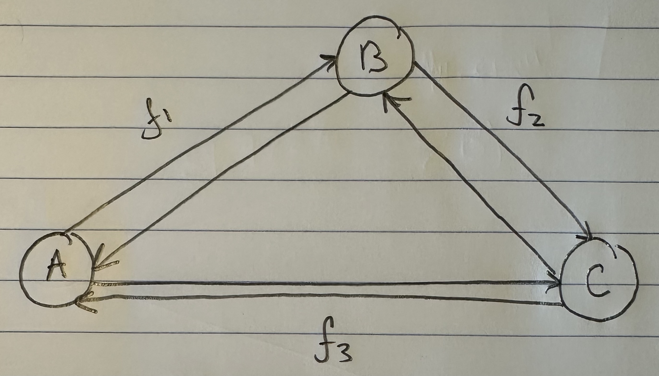
We can improve our measure of K-complexity by noting that any graph can be described by simply listing its edges. For example, a complete graph on three vertices can be represented by the set of vectors $E = \{(1,2), (2,3), (3,1)\}$ . That is, each vector represents an edge, and the digits in the vector tell you the labels of the vertices connected by the edge in question. In this case $E$ connects vertex $1$ to $2$ , $2$ to $3$ , and $3$ to $1$ , producing a circuit on three vertices, i.e., a complete graph on three vertices. As a consequence, the K-complexity of a graph cannot exceed the complexity of its edge set. Each label in a graph will be less than the order of the graph (i.e., the number of vertices $N$ ), and as a result, we can encode each label in the edge set with at most $\log(N)$ bits. Each edge consists of two labels, and so the K-complexity of a graph must be less than or equal to $|E| 2\log(N) + C$ .

Structural Complexity

Note that $|E| 2\log(N)$ is again an upper bound on the K-complexity of a graph, it’s just much better than $N^2$ , since it at least takes into account the number of edges, and uses a more efficient representation of the graph. However, particular graphs can definitely be expressed in fewer bits. Specifically, the empty graph, the complete graph, and a Hamiltonian circuit, each of a given order $N$ , can be expressed in $\log(N) + C$ bits, where $C$ is a constant that is the length of the program that constructs the graph, which we can think of as simply generating the list of edges that defines the graph. For example, the following Octave Code will generate a Hamiltonian circuit of any order $N$ :

E{1} = (1,N);

for i = 2 : N – 1

E{i} = (i, i+1);

endfor

As a result, we can produce a Hamiltonian circuit of any order, using at most $\log(N) + C$ bits, where $C$ is the length of the program above in bits. Analogous code will produce a complete graph, whereas an empty graph can be produced by simply specifying $N$ (i.e., there are no edges), which again requires exactly $\log(N) + C$ bits, but using different code. Note that even in these cases, it’s still possible that an even shorter, presumably not universal program produces a given graph as its output when fed as the input to a UTM. That is, e.g., $U(x) = M(G)$ , where $x$ is a binary string, $U$ is some UTM, and $M(G)$ is the matrix that defines the graph $G$ . As a theoretical matter, the length of $x$ could be even smaller than $\log(N)$ , where again $N$ is the order of $G$ . This would be true for empty graphs, complete graphs, and Hamiltonian circuits of order $N$ , where the number $N$ itself is highly compressible.

Kolmogorov-Random Graphs

It turns out it’s pretty easy to prove that Kolmogorov-Random Graphs exist, in the sense that we can produce graphs using Kolmogorov-Random strings. There’s obviously scholarship on point, but I think the ideas I’ve set out in this note are a lot easier to think about, and unify perfectly with the complexity of strings. Specifically, recall that we can represent any graph using its edge set. If we modify the method used to do so above, we can show that Kolmogorov-Random strings will produce graphs when fed as inputs to a UTM, which implies that those graphs are literally Kolmogorov-Random, in the same sense as a binary string.

Returning to the example of a complete graph on three vertices above, let’s represent that graph using three sets: the set of vertices adjacent to $v_1$ , the set of vertices adjacent to $v_2$ , and the set of vertices adjacent to $v_3$ . Because it’s a complete graph on three vertices, we would have the following: $\{v_2\}, \{v_3\}, \{v_1\}$ . Note that as we move forward in the labels, e.g., from vertex $1$ to vertex $2$ , we gain information about the graph. Specifically, there’s no reason to include $v_1$ in the set of vertices adjacent to $v_2$ , since that information is contained in the set of vertices adjacent to $v_1$ . As a result, the maximum number of elements in the set for $v_1$ is $N-1$ , and for $v_2$ it’s $N-2$ , and so on. As a result, we can represent the graph as a “matrix” where the number of columns begins at $N-1$ for $v_1$ , and decreases by $1$ for each row. Note that as a result, the $N$ -th row has no columns, implying that the “matrix” has $N-1$ rows. We can treat every entry in this “matrix” as a binary number indicating the presence or absence of a given edge. For example, if entry $(1,3)$ is $1$ , then edge $(1,3)$ is included in the graph. This is just like a regular graph matrix, except it contains no duplicate entries, and therefore the number of columns is not constant. Note that therefore, it corresponds to a binary string of length $(N - 1) + (N - 2) + \ldots + 1 = \frac{N (N - 1)}{2} =$ $N \choose 2$ , which is also the maximum number of edges.

Let $s$ be a Kolmogorov-Random string of length $N =$ $n \choose 2$ . All we have to do is restructure $s$ into the shape of a “matrix” described above, which will produce a graph $G$ . Because $s$ is Kolmogorov-Random, there cannot be another binary string shorter than $s$ that will generate $G$ on a UTM, by which we mean generating the edges of $G$ . Assume such a string $y$ exists. It follows that $E(G) = U(y)$ , which in turn will allow us to construct a “matrix” of the type above, which will in turn produce $s$ . Because $s$ is Kolmogorov-Random, there cannot be a string shorter than $s$ that generates $s$ , yet $y$ is exactly such a string, which produces a contradiction, completing the proof.

Note that such a graph $G$ cannot be a complete graph, since a complete graph has a trivial complexity, as we’ve seen above. It is therefore interesting that a Kolmogorov-Random Graph has a Kolmogorov Complexity of exactly the number of edges in a complete graph of the same order. Because not all numbers are of the form $N =$ $n \choose 2$ , we cannot say that the Kolmogorov Complexity of a Kolmogorov Random graph is always the number of edges in a complete graph of the same order, though it might nonetheless be true.

Computability and Infinite Sets of Graphs

Let $H_N$ denote the Hamiltonian circuit of order $N$ , and let $\Gamma = \{H_1, H_2, \ldots \}$ . Despite the fact the set is infinite, because each such graph has a simple structure, we can define a computable test that will allow us to determine whether a graph $G$ is in that set, or not. Just to sketch the algorithmic test, we would begin by testing the degree of each vertex in $G$ , and if it’s not $2$ , the algorithm terminates and returns “false”. If the degree of each vertex is in fact $2$ , then we traverse the edges of the graph, and if we don’t return to the original vertex, we again return “false”, otherwise we return “true”. As a result, there is a computable test that allows us to state whether or not a given graph $G$ is in $\Gamma$ . Note that as a consequence, we can also generate $\Gamma$ , using brute force, producing all graphs of orders $N = 1, 2, \ldots$ and testing which of those belong in $\Gamma$ . Similarly, as noted above, we can algorithmically construct a Hamiltonian circuit of all orders, and can therefore, test whether or not a given graph is in the set of graphs generated by that process. Note that the constructive algorithm above, is very different from the algorithmic test we just articulated in this section. Therefore, we have an interesting equivalence, in that the existence of an algorithmic test implies a constructive algorithm (via brute force), and a constructive algorithm implies an algorithmic test (again via brute force, e.g., in the case where there are multiple graphs of a given order).

At the same time, because the set of graphs is countably infinite, and the set of algorithms is countably infinite, the number of infinite subsets of the set of all graphs is uncountable and therefore larger than the set of all algorithms. Therefore, it must be the case that there are infinite sets of graphs that do not have an algorithmic test, and therefore do not have a constructive algorithm. One simple example follows from the existence of non-computable infinite strings. Again, the set of all infinite binary strings is uncountable, whereas the set of all algorithms is countable. As a consequence, there must be infinite strings that cannot be generated by a finite program running on a UTM.

Let $\sigma$ be such a non-computable infinite string. Define $\bar{\Gamma}$ as the subset of $\Gamma$ such that $H_i$ is included in $\bar{\Gamma}$ if $\sigma(i) = 1$ . That is, where $\sigma(i) = 1$ , we include the corresponding element of $\Gamma$ . As noted above, there is a simple algorithmic test to determine whether or not each element of $\bar{\Gamma}$ is Hamiltonian, but this is distinct from an algorithmic test that determines whether or not a given graph $G$ , is in $\bar{\Gamma}$ . That is, not all Hamiltonian circuits are in $\bar{\Gamma}$ . Now assume that such an algorithmic test $T$ exists. It follows that we can then generate every Hamiltonian circuit starting with $N = 1$ , and $T$ will tell us whether or not that particular order is included in $\bar{\Gamma}$ . If $H_i$ is included, set binary string entry $\zeta(i) = 1$ and otherwise set $\zeta(i) = 0$ . It follows that $\zeta = \sigma$ . However, we generated $\zeta$ on a UTM, which is not possible, since $\sigma$ is by definition non-computable, which leads to a contradiction. This implies $T$ does not exist. This demonstrates that even if a set is computable, it will have non-computable subsets, just like the natural numbers, and all countable sets generally.

Properties without Computable Tests

In the previous section I noted that Hamiltonian circuits are simple structures, and therefore, we can come up with simple algorithms that test for whether or not a graph is a Hamiltonian circuit. Testing whether or not a given graph contains a Hamiltonian circuit as a subgraph is believed to be intractable. As such, there are simple structures that correspond to simple algorithms, though finding simple structures in more complex graphs is suddenly intractable. This raises the question of whether or not there are properties that cannot be tested for algorithmically at all. The answer is yes.

Order the set of all finite graphs $G_1, G_2, \ldots$ , and let $\gamma$ be an infinite binary string. If $\gamma(i) = 1$ , then we can interpret this as $G_1$ having property $\gamma$ given the ordering, or equivalently, view $\gamma$ as defining a set of graphs. There are again more binary strings than there are algorithms, and therefore, in this view, more properties than there are algorithms. The question is whether there are more interesting and / or useful properties than there are algorithms, but the bottom line is, the number of properties is uncountable, and therefore the density of testable properties is zero. You might be tempted to say that all such properties are uninteresting, or not useful, but unfortunately, whether or not a program will halt is precisely one of these properties, which is both useful and interesting, suggesting at least the possibility of other such useful and interesting properties.

The Distribution of Graph Properties

Ramsey Theory is one of the most astonishing fields of mathematics, in particular, because like all combinatorics, it has intrinsic physical meaning, in that combinatorics provides information about the behavior of reality itself. What’s astonishing about Ramsey Theory in particular, is that it’s fair to say that it shows that structure increases as a function of scale, in that as objects get larger, they must have certain properties. What I realized today, is that the number of properties that they can have also grows as a function of scale. For intuition, consider all graphs on $N = 1,2,3$ vertices. You can see right away that the complete graph on $3$ vertices is the smallest possible Hamiltonian circuit, and therefore, the smallest Hamiltonian graph. It is simply not possible to have a Hamiltonian graph with fewer vertices. This suggests the possibility that the number of properties that a graph can have grows as a function of its order, and we show using some not terribly impressive examples, that this in fact must be true, suggesting the possibility, that useful and interesting properties of objects continue to arise as a function of their scale.

Let $\gamma$ be an infinite binary string, and define an infinite subset of the natural numbers $A$ such that $k \in \mathbb{N}$ is included in $A$ if $\gamma(i) = 1$ . Now define an infinite set of graphs $\Gamma$ such that $H_i$ is in $\Gamma$ if the number of edges of $H_i$ is divisible by $A(i)$ . Because each $H_i$ is a Hamiltonian circuit, the number of edges in $H_i$ is simply $i$ . Putting it all together, we have an infinite set of graphs, each of which are Hamiltonian circuits of different orders, and whether or not a given order is included in the set, is determined by whether or not that order is divisible by the corresponding integer value in $A$ . Note that larger graphs will have orders that are divisible by more numbers, though the number of divisors does not increase monotonically as a function of $n \in \mathbb{N}$ . Therefore, in this view, larger graphs have more properties in the sense of being included in more sets of this type.

Complexity Versus Computability

Intuitively, there is a connection between complexity and computability. In at least one case, this is true, in that the Kolmogorov Complexity of a non-computable infinite string is countable. That is, if a string is non-computable, then there is no finite input to a UTM that will generate that string. As a result, its complexity cannot be finite. At the same time, we can simply copy the string from the input tape, to the output tape, assuming both are infinite tapes. Therefore, the Kolmogorov Complexity of a non-computable infinite string is countable. However, this intuition is subject to more careful examination in the case of infinite sets, in that you can construct non-computable sets of low-complexity objects.

Now assume that $\gamma$ from the example in the previous section is non-computable, which implies that both $A$ and $\Gamma$ are non-computable. As discussed above, it follows that there is no computable test for inclusion in $\Gamma$ . At the same time, each of the graphs in $\Gamma$ is a Hamiltonian circuit, with a Kolmogorov Complexity of $\log(N) + C$ . Note that the ratio $\frac{\log(N)}{{N \choose 2}}$ approaches zero as $N$ approaches infinity. As such, we have an infinite set of graphs that is non-computable, but each of the individual graphs are low-complexity objects, though note that the set was generated using a non-computable string.

Ancestry Test Code

February 26, 2024March 16, 2024 / erdosfan / Leave a comment

As I’ve noted several times, I’ve devised an ancestry test that is impossible to argue with, using whole-genome mtDNA. See Section 6.1 of A New Model of Computational Genomics [1]. Specifically, given whole-genomes A, B, and C, if genome A is the ancestor of both genomes B and C, then it must be the case with near certainty that genomes A and B, and A and C, have more bases in common than genomes B and C. Again, see [1] for an explanation. The test in Section 6.1 of [1] is at the genome level, and as such, using a dataset of genomes, the number of tests required to compare whether an entire population is the ancestor of two other populations grows quickly as a function of population sizes. As a tractable approximation, the attached code uses the average match count between populations A and B, A and C, and B and C, which of course loses information, but should at least help you reduce the number of cases that you investigate exhaustively.

Applying the attached, it turns out, that yet again, the Denisovans test as the common ancestor of humanity (though I now think the Cameroon might be more modern than I first suspected), specifically, the common ancestor of both Heidelbergensis and Neanderthals. Further, the Phoenicians again test as the common ancestor of basically everyone alive today, including the modern Thai, Nigerians, Norwegians, Koreans, the Saqqaq (in B.C. Greenland!), the Swedes, Indians, and Chinese. As a result, I’m fairly convinced early Middle Eastern people settled a significant portion of Europe and Asia, and possibly America (given Greenland), but I can’t put a date on it. Ugarit goes back to 6,000 BC, which should leave enough time, but this is an ordinal test only, and therefore cannot be used to date the relationships. Moreover, I’ve recently cast serious doubt on the idea that mtDNA has a single, stable rate of mutation. The net point is, therefore, the ancestry test is real, and very difficult to argue with, but limited to ordinal testing; further, mtDNA doesn’t seem to have a single, stable rate of mutation; as a result, it looks plausible (1) that the Denisovans are the first humans and (2) that either the Phoenicians or people close to them (on the maternal line) we’re prolific settlers, but we don’t know when either got started.

The code is below, the balance can be found in [1]. One modification I plan to make is to use Monte-Carlo probing on the data that informs the averages. This will allow you to test a fixed portion of the genome-level data that you can scale given the power of your machine. BTW I just bought a Mac Mini running the M2 Pro chip, and I cannot recommend this machine enough, it is more than 10 times faster than my windows laptop. Running the ancestry test described above over 673 full mtDNA genomes takes about 0.5 seconds. I cannot believe this is a retail machine.

class-based-ancestry-algorithm Download