Summary

My core work in deep learning makes use of a notion that I call , which is the minimum distance over which distinction between two vectors is justified by the context of the dataset. As a consequence, if you know , then by retrieving all vectors in the dataset for which , you can thereby generate a cluster associated with the vector . This has remarkable accuracy, and the runtime is , where is the number of rows in the dataset, on a parallel machine. You can read a summary of the approach and the results as applied to benchmark UCI and MNIST datasets in my article, “Vectorized Deep Learning“.

Though the runtime is already fast, often fractions of a second for a dataset with a few hundred rows, you can eliminate the training step embedded in this process, by simply estimating the value of using a function of the standard deviation. Because you’re estimating the value of , the cluster returned could very well contain vectors from other classes, but this is fine, because you can then use the distribution of classes in the cluster to assign a probability to resultant predictions. For example, if you query a cluster for a vector , and get a cluster , and the mode class (i.e., the most frequent), has a density of within , then you can reasonably say that the probability your answer is correct is . This turns out to not work all the time, and very well sometimes, depending upon the dataset. It must work where the distribution of classes about a point is the same in the training and testing datasets, and this follows trivially from the lemmas and corollaries I present in my article, “Analyzing Dataset Consistency“. But of course, in the real world, these assumptions might not hold perfectly, which causes performance to suffer.

Another layer of analysis you can apply that allows you to measure the confidence in a given probability makes use of my work in information theory, and in particular, the equation,

,

where is the total information that can be known about a system, is your Knowledge with the respect to the system, and is your Uncertainty with respect to the system. In this case, the equation reduces to the following:

,

where is the size of the prediction cluster, is the number of classes in the dataset, is again Knowledge, and is the Shannon Entropy of the prediction cluster, as a function of the distribution of classes in the cluster.

You can then require both the probability of a prediction, and your Knowledge in that probability, to exceed a given threshold in order to accept the prediction as valid.

Knowledge is in this case given by,

.

You can read about why these equations make sense in my paper, “Information, Knowledge, and Uncertainty“.

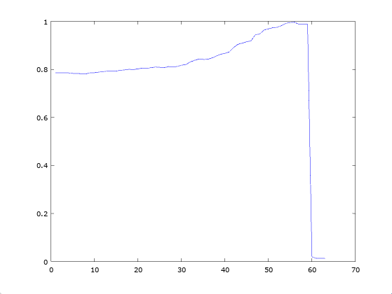
If you do this, it works quite well, and below is a plot of accuracy as a function of a threshold for both the probability and Knowledge, with Knowledge adjusted to an scale, given rows of the MNIST Fashion Dataset. The effect of this is to require an increasingly high probability, and increasing confidence in your measure of that probability. The dataset is then broken into random training and random testing rows, done times. The accuracy shown below is the average over each of the runs, as a function of the minimum threshold, which is again, applied to both the accuracy and the confidence. The reason the prediction drops to at a certain point, is because there are no rows left that satisfy the threshold. The accuracy peaks at , and again, this is without any training step, so it is in fairness, an unsupervised algorithm.

The results are comparable for the MRI Brain Cancer Dataset (max accuracy of 100%), Harvard Skin Cancer Dataset (max accuracy of 93.486%).

This method is already baked into some of my most recent posts, but I wanted to call attention to it in isolation, because it is interesting and useful. Specifically, my algorithms are generally rooted in a handful of lemmas and corollaries that I introduced, that prove, that the nearest neighbor method produces perfect accuracy, when classifications don’t change over small fixed distances. That is, if I’m given a row vector from the dataset, and the set of points near have the same classifier as , then the nearest neighbor algorithm can be modified slightly to produce perfect accuracy. And I’ve introduced a ton of software that allows you to find that appropriate distance, which I call . The reason this sort of new approach (I came up with this a while ago) is interesting, is because it doesn’t require any supervision –

It uses a fixed form formula to calculate , as opposed to a training step.

This results in a prediction algorithm that has runtime, and the accuracy is consistently better than nearest neighbor. Note that you can also construct an runtime algorithm using the code attached to my paper Sorting, Information, and Recursion.

Here are the results as applied to the MNIST Fashion Dataset using 7,500 randomly selected rows, run 500 times, on 500 randomly selected training / testing datasets:

1. Nearest Neighbor:

Accuracy: 87.805% (on average)

2. Cluster-Based:

Accuracy: 93.188% (on average)

Given 500 randomly selected training / testing datasets, the cluster-based method beat the accuracy of nearest neighbor method 464 times, the nearest neighbor method beat the cluster-based method 0 times, and they were equal 36 times. The runtime from start to finish is a few seconds (for a single round of predictions), including preprocessing the images, running on an iMac.

NOTE: there is an error in the code, that I am deliberately leaving, because I can’t explain why accuracy actually increases as the code is written, as a function of confidence. I’m working on something else at the moment, post coming soon, but I wanted to flag the error, and the related apparent mystery. In short, the code as written returns the cluster for a random row of the dataset, rather than the row that the input vector mapped to.

Attached is code that implements information-based measures of confidence, that allows you to filter predictions based upon confidence, in turn improving accuracy. Below are two images, one showing the total number of errors for each class of the dataset as a function of confidence (on the left), and another showing overall accuracy as a function of confidence (on the right), each as applied to the Harvard Skin Cancer Dataset, which I’ve found to be awful, as the images are not consistent, and one class makes up basically all of the data.

In each case, prediction was run 1,000 times, using 1,000 randomly generated training and testing datasets, comprised of 350 rows, which is a very small subset of the roughly 10,000 rows of the dataset. This is why the number of errors begins in the thousands, because it is the total over all runs (bottom image). In contrast, the accuracy is the average accuracy at a given level of confidence (x-axis) over all runs (top image). The purpose of this initial note is to demonstrate that the measure of confidence works, and later, I will run the same simulation on the full dataset, to demonstrate that not only does the measure of confidence work, but it also works in solving practical datasets, increasing accuracy. In any case, because it was a such a challenging dataset, it lead to this implementation, which was ultimately a good thing.

The fundamental principle underlying the measure of confidence, is the equation I introduced a while back, which is , where is information, is knowledge, and is uncertainty. In this case, confidence in a prediction is given by . I’ll explain how those values are calculated later, but you can look through the code to see they’re related to entropy and information theory generally. The equation states something that must be true about epistemology, which is that the sum of what you know about a system (), and what you don’t know about the system(), must be the sum total of information regarding the system (). What’s interesting in this application, is that using information theory and combinatorics, we can actually solve for all three variables, and empirically, it works, at least in the case of this dataset. I don’t think you can ever prove that you’ve used the correct values for these variables, but you can use information theory to derive objective values for all three variable.

I’m going to write something formal over the coming week, but in the short run, here are the runtime and accuracy results of the methods introduced in a prior article on medical imaging classification using my software, as applied to a Skin Cancer Dataset from Harvard.

Summary of Results

Original Dataset Size: 7470 RGB images of various dimensions;

Compressed Dataset Size: 7470 x 198;

Preprocessing time: 37.9 seconds;

Supervision Training time: 55.9 seconds;

Prediction time: 13 seconds, on average (run 25 times);

Prediction accuracy:

Worst case, 85.542% (no supervision);

Best case, 95.8337% (highest level supervision, rejecting all but 62 rows).

Bottom line: Reliable diagnosis for over 7,000 patients, on a home computer, in about 2 minutes.

Summary of Process

The dataset consists of just over 10,000 images of legions. Each legion belongs to one of seven classes of legions, three of which are malignant. The algorithm consolidates all malignant classes into one, and consolidates all benign classes into one. It removes all duplicate images, leaving only one image per patient. All images are then compressed, and fed to a supervised algorithm that finds the minimum and maximum distances over which classification labels are consistent within the dataset. Then prediction is applied using decreasingly sensitive criteria for flagging predictions as outside the scope of the training dataset.

I’ve also attached a “STAT SUPERVISION” script that can be applied without consolidating classes, and generates about 80% accuracy (also using rejections). This is the same algorithm I introduced in Section 1.4 of this paper, for the “Statistical Spheres” dataset, the only difference here is the clusters don’t have the same classifier, but the algorithm is exactly the same.

There’s another method called “Isolate Classes”, the code for which is also attached, that I’ll explain fully in a separate post (that doesn’t quite yet work), which was actually the original approach, which is to isolate a single class, and try to identify which rows are in that class. This works out nicely on parallel machines, because you run tests for each class simultaneously, but this is not something you can do on a PC.

Code:

I’ve just applied my basic supervised image classification algorithm (see Section 1.2 of this paper) to an MRI image classification dataset from Kaggle, and a Skin Cancer classification dataset from Harvard. The MRI Dataset classification task is to classify the type of brain tumor, or absence thereof, given four classes. The accuracy for the MRI Dataset is consistently around 100% (using randomized partitions into training / testing datasets), and the runtime over 1503 training rows is 15 seconds (including pre-processing) running on an iMac.

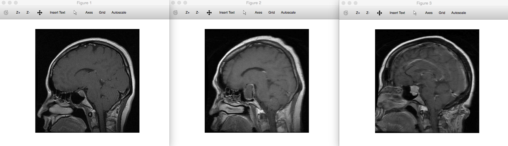
I’ve also applied the supervised clustering algorithm (see the same paper above) to the MRI dataset, which has an accuracy around 94%. This would allow doctors to not only diagnose patients with great accuracy on a cheap computer, since the clustering step would also allow them to compare the most similar brain scans. Clustering the entire testing dataset of 376 rows in this case took about 10 seconds, running on an iMac. For example, the left most image above is an input image of a pituitary brain tumor, and the two images to the right of that are the images returned by the clustering algorithm, both of which also represent brains with pituitary tumors.

The downside to my approach is that the algorithm “rejects” a large number of rows from the testing dataset as outside of the scope of the training dataset (always on a blind basis, based upon only training data). Without getting too into details, you can soften the standard it uses to reject data, and if you do so, of course, the percentage of rows that gets rejected starts to decrease, though accuracy starts to suffer.

So what I’ve done for the Skin Cancer dataset is to allow a sliding scale of precision, that rejects fewer and fewer rows, and reports the classification prediction accuracy at each scale. This lets the user decide whether they want basically perfect confidence in their predictions, at the expense of rejecting a large portion of the testing dataset, or somewhere just beyond that, perhaps significantly so, if they’re more interested in bulk predictions than precision. For the Skin Cancer Dataset, this produces accuracies that range from 100%, with a rejection rate of 99.750%, to 85.750%, with a rejection rate of 0%, which is effectively unsupervised nearest neighbor. Note that I’ve consolidated all of the malignant classes into one class, leaving the benign class as the second class. I’ve also converted the dataset to grey scale, so it’s possible you’d get even better accuracy using full color, since from what I understand, color is relevant to classifying skin lesions. You could tweak these techniques, to, for example, reduce the rejection rate until it hits zero, whereas I’ve used a fixed number of iterations for simplicity, for now.

Finally, note that the Skin Cancer dataset contains not proper duplicates, but at times multiple photos of the same patient’s lesions, so as a temporary fix, I’ve randomly selected a subset of the total dataset, which means the issue shouldn’t occur too often, since the number of rows selected is 2000, out of roughly 10,000, and the number of duplicates is typically 2 or 3. I’ve already fixed this formally, by selecting exactly one image for each patient, and the accuracy was unchanged. I’m now working on the full dataset of one image per patient, which is taking some time to process, because it’s large, but the updated code should be up by tomorrow.

In general, this method should work for any single image classification dataset, where physical structure, or coloring, is indicative of disease. I will write a formal paper on the topic shortly.

The implications here are dramatic, and could democratize advanced healthcare  –

All you need is a cheap laptop, the applicable dataset, and my software, and it seems, you can diagnose at least some conditions en mass, with great reliability, in just a few minutes. This would allow doctors to focus on only those patients that test positive, or have their results flagged as outside of the dataset, in this case reducing the caseload significantly. This is a big deal when you’re talking about a large number of people. By the same logic, this software allows you to reliably diagnose thousands of people, in a few minutes, again, with high accuracy.

You should run this on my updated algorithms, available on ResearchGate.

Here’s the command line code in Ocatve / Matlab:

I’ve done a ton of work on complexity of motion and gestures, some specifically applied to robotics, and a lot of it unpublished, which annoyed me, but I’m pleased that the paper I just got up and running (not quite final yet), Sorting, Information, and Recursion, includes an equation that is plainly the culmination of this work, and would allow you to measure the entropy of a sequence of motions, which can be found in Equations (1) and (2) of the paper.

Specifically, simply represent the velocity of a system over time as a sequence of velocity vectors , and if you can express the differences between all adjacent vectors as either a real number or a real number vector, then you can use the equations in that paper to calculate an order dependent analog of entropy, that I discuss in some detail. It behaves exactly the way you’d want, which is if motions are highly volatile in sequence, you get a higher entropy, and if the velocity is constant, you get a zero entropy. I discuss this in more detail in the paper, and in particular, in Footnotes 5 and 6.

You can look at it three ways: (1) take the sequence as it is observed, (2) sort it, which will minimize the entropy (see Corollary 3.1), or (3) apply another ordering that will maximize the entropy (see Footnote 8). These three measures tell you (1) what the real sequence entropy is, (2) what its theoretical minimum is, and (3) what its theoretical maximum is. This could be useful where you don’t have total control of the sequence itself, and instead can only set the individual velocities, giving you an objective criteria that would allow you to compare the complexities of two sets of motions. The lower the entropy, the smoother the motion should look to an observer, which is important not just for robotics, but also all modes of transportation, where people naturally feel frightened by sudden acceleration.

Just imagine monitoring the programs running over time on a CPU. It is obviously common to have multiple programs running at the same time, though typically you have only one program that is contained in some active window. However, even though a program is in the background, it will still enter the processor from time to time. As a result, we can imagine the programs coming in and out of the processor over time as a sequence expressed as a vector . Note that because there will likely be only one active window at a time, there will probably be some program that appears most often in memory, over any given period of time, though this isn’t terribly relevant to the more general concept I’m introducing, which is comparing sequences of labels. Specifically, in this case, it doesn’t mean anything to take the difference between and , because they’re just labels that don’t have any intrinsic numerical value.

Nonetheless, we could for many reasons want to compare two sequences of labels. For example, just imagine some programs use more electrical power than others. You could for this reason, want to compare two sequences of labels so that you could predict what programs will follow, or how long a given program will remain open, etc. This would in turn, allow you to predict power consumption, CPU usage, battery life, etc. And I came up with a method earlier today that is quite simple, and allows you to compare arbitrary sequences of labels that can be different lengths, and contain different labels.

I’ll begin by example to establish an intuition, so let and let . Note that we are not treating the entries of the sequences as numbers, but instead as labels, so we could have used “apple”, “orange”, “quince”, rather than numbers, as it doesn’t matter, and you’ll see why in just a moment. The sequence is longer than , so let’s begin with , and begin with the first element . We then search for in sequence , to find that it is in exactly the same index, and so we assign it a score of 1, as if it contributed 1 full element to the intersection of two sets, and so the total pseudo-intersection score between and is thus far now 1. We then search for , as it is the second element of , to find that it is in index 3 of sequence . Because it is not in exactly the same index, we treat it as contributing less than 1 full element to the pseudo-intersection of sequences and . You could do this differently, but the equation I’m going to use is as follows:

,

where is the distance between the indexes in question. So in this case, because the from sequence is in index 2, and the from sequence is in index 3, , and so the pseudo intersection score is . If we continue this process, we produce a total pseudo-intersection of , since the second from is in index 3, and does not exist in sequence . As is evident, the further away a given entry is from a corresponding entry, the less it contributes to the total pseudo-intersection, and if it’s not there at all, then it contributes nothing.

This would allow you to use my intersection clustering software to cluster these types of sequences, and make predictions (maximally intersecting sequences are the nearest neighbors of each other), but more interesting than that, this makes some sense of fractional cardinalities, which is something I’ve been working on lately in the context of the logarithm of fractions. Specifically, the information capacity of a system that can be in states, is , but what does it mean for a system to have a fractional number of states? You could view it as Quantum Superposition, since you could say, every unit of energy within the system is subdivided among more than one state, meaning the energy of the system is always subdivided beyond unity, producing a fractional number of states for each unit of energy. You could also, say it’s the result of a pseudo-intersection of this type, that doesn’t really have any clear physical meaning, but has a mathematical meaning, as described above.

In any case, you can plainly use this technique to predict draws on capacity of all types, from food inventories and electricity to CPU’s themselves, and though it doesn’t offer any obvious means of making batteries or processors more efficient, the reality is, planning always allows for more efficiency.

I’ve just finished another short book of poetry, that is dedicated to an ostensibly fictional character in my book VeGa. The poetry is what it is, but like a lot of what I write, it plainly draws upon Chan Buddhism.

Enjoy!

James’s song

I’ve updated the paper that discusses some of the recent results I’ve proved on this blog, to include heavily annotated code, given that there seems to have been some confusion about the runtime of the algorithms on reddit.

The results prove that (1) a list is sorted if and only if the distance between adjacent entires is minimized, and (2) a list is sorted if and only if an encoding of the list as a particular class of recurrence relation minimizes information. These results together demonstrate an equivalence between sorting and minimizing information, which is in my opinion, non-obvious. I also introduced what I believe to be the fastest known sorting algorithms, one with an runtime, and another with an runtime, both of which are already faster than the lower bounds of for serial sorting algorithms (both algorithms are parallel). The code for both are attached to the paper linked to above, which you can also find below.

 

I’ve combined some of my recent work on sorting and information theory into a single formal paper, available on ResearchGate.