In a previous post below entitled, “Image Recognition with No Prior Information”, I introduced an algorithm that can identify structure in random images with no prior information by making use of assumptions rooted in information theory. As part of that algorithm, I showed how we can use the Shannon entropy of a matrix to create meaningful, objective categorizations ex ante, without any prior information about the data we’re categorizing. In this post, I’ll present a generalized algorithm that can take in an arbitrary data set, and quickly construct meaningful, intuitively correct partitions of the data set, again with no prior information.

Though I am still conducting research on the run-time of the algorithm, the algorithm generally takes only a few seconds to run on an ordinary commercial laptop, and I believe the worst case complexity of the algorithm to be , where n is the number of data points in the data set.

The Distribution of Information

Consider the vector of integers  x = [1 2 3 5 10 11 15 21]. In order to store, convey, or operate on x, we’d have to represent x in some form, and as a result, by its nature, x has some intrinsic information content. In this case, x consists of a series of 8 integers, all less than , so we could, for example, represent the entire vector as a series of 8, 5-bit binary numbers, using a total of 40 bits. This would be a reasonable measure of the amount of information required to store or communicate x. But for purposes of this algorithm, we’re not really interested in how much information is required to store or communicate a data set. Instead, we’re actually more interested in the information content of certain partitions of the data set.

Specifically, we begin by partitioning x into equal intervals of Δ = (21-1) / N, where N is some integer. That is, we take the max and min elements, take their difference, and divide by some integer N, which will result in some rational number that we’ll use as an interval with which we’ll partition x. If we let N = 2, then Δ = 10, and our partition is given by {1 2 3 5 10 11} {15 21}. That is, we begin with the minimum element of the set, add Δ, and all elements less than or equal to that minimum + Δ are included in the first subset. In this case, this would group all elements from 1 to 1 + Δ = 11. The next subset is in this case generated by taking all numbers greater than 11, up to and including 1 + 2Δ = 21. If instead we let N = 3, then Δ = 6 + ⅔, and our partition is in this case given by {1 2 3 5} {10 11} {15 21}.

As expected, by increasing N, we decrease Δ, thereby generating a partition that consists of a larger number of smaller subsets. As a result, the information content of our partition changes as a function of N, and eventually, our partition will consist entirely of single element sets that contain an equal amount of information (and possibly, some empty subsets). Somewhere along the way from N = 1 to that maximum, we’ll reach a point where the subsets contain maximally different amounts of information, which we treat as an objective point of interest, since it is an a priori partition that generates maximally different subsets, at least with respect to their information content.

First, we’ll need to define our measure of information content. For this purpose, we assume that the information content of a subset is given by the Shannon information,

,

where p is the probability of the subset. In this case, the partition is a static artifact, and as a result, the subsets don’t have real probabilities. Nonetheless, each partition is by definition comprised of some number of m elements, where m is some portion of the total number of elements M. For example, in this case, M = 8, and for Δ = 6 + ⅔, the first subset of the partition consists of m = 4 elements. As a result, we could assume that p = m/M = ½, producing an information content of log(2) = 1 bit.

As noted above, as we iterate through values of N, the information contents of the subsets will change. For any fixed value of N, we can measure the standard deviation of the information contents of the subsets generated by the partition. There will be some value of N for which this standard deviation is maximized. This is the value of N that will generate maximally different subsets of x that are all nonetheless bounded by the same interval Δ.

This is not, however, where the algorithm ends. Instead, it is just a pre-processing step we’ll use to measure how symmetrical the data is. Specifically, if the data is highly asymmetrical, then a low value of N will result in a partition that consists of subsets with different numbers of elements, and therefore, different measures of information content. In contrast, if the data is highly symmetrical, then it will require several subdivisions until the data is broken into unequally sized subsets.

For example, consider the set {1, 2, 3, 4, 15}. If N = 2, then Δ = 7, and immediately, the set set is broken into subsets of {1, 2, 3, 4} and {15}, which are of significantly different sizes when compared to the size of the original set. In contrast, given the set {1, 2, 3, 4, 5}, if N = 2, then Δ = 2, resulting in subsets of {1, 2, 3} {4, 5}. It turns out that the standard deviation is in this case maximized when N = 3, resulting in a partition given by {1, 2} {3} {4, 5}. We can then express the standard deviation of the partition as an Octave vector:

std( [ log(5/2) log(5) log(5/2) ] ) = 0.57735.

As a result, we can use N as a measure of symmetry, which will in turn inform how we ultimately group elements together into categories. The attached partition_vec script finds the optimum value of N.

Symmetry, Dispersion, and Expected Category Sizes

To begin, recall that N can be used as a measure of the symmetry of a data set. Specifically, returning to our example x = [1 2 3 5 10 11 15 21] above, it turns out that N = 2, producing a maximum standard deviation of 1.1207 bits. This means that it requires very little subdivision to cause x to be partitioned into equally bounded subsets that contain maximally different amounts of information. This suggests that there’s a decent chance that we can meaningfully partition x into categories that are “big” relative to its total size. Superficially, this seems reasonable, since, for example, {1 2 3 5} {10 11 15} {21} would certainly be a reasonable partition.

As a general matter, we assume that a high value of N creates an ex ante expectation of small categories, and that a low value of N creates an ex ante expectation of large categories. As a result, a high value of N should correspond to a small initial guess as to how different two elements need to be in order to be categorized separately, and a low value of N should correspond to a large initial guess for this value.

It turns out that the following equation, which I developed in the context of recognizing structure in images, works quite well:

,

where divisor is the number by which we’ll divide the standard deviation of our data set, generating our initial minimum “guess” as to what constitutes a sufficient difference between elements in order to cause them to be categorized separately. That is, our initial sufficient difference will be proportional to s / divisor.

“Symm” is, as the name suggests, yet another a measure of symmetry, and a measure of dispersion about the median of a data set. Symm also forms the basis of a very simple measure of correlation that I’ll discuss in a follow up post. Specifically, symm is given by the square root of the average of the sum of the squares of the differences between the maximum and minimum elements of a set, the second largest and second smallest element of a set, and so on.

For example, in the case of the vector x, symm is given by,

which is 12.826.

As we increase the distance between the elements from the median of a data set, we increase symm. As we decrease this distance, we decrease symm. For example, symm([ 2 3 4 5 6 ]) is greater than symm([ 3 3.5 4 4.5 5 ]). Also note that a data set that is “tightly packed” on one side of its median and diffuse on the other will have a lower value of symm than another data set that is diffuse on both sides of its median. For example, symm([ 1 2 3 4 4.1 4.2 4.3 ]) is less than symm([ 1 2 3 4 5 6 7 ]).

For purposes of our algorithm, symm is yet another a measure of how big we should expect our categories to be ex ante. A large value of symm implies a data set that is diffuse about its median, suggesting bigger categories, whereas a small value of symm implies a data set that is tightly packed about its median, suggesting smaller categories. For purposes of calculating divisor above, we first convert the vector in question into a probability distribution by dividing by the sum over all elements of the vector. So in the case of x, we first calculate,

x’ = [0.014706 0.029412 0.044118 0.073529 0.147059 0.161765 0.220588 0.308824].

Then, we calculate symm(x’) = 0.18861. Putting it all together, this implies divisor = 0.30797.

Determining Sufficient Difference

One of the great things about this approach is that it allows us to define an objective, a priori measure of how different two elements need to be in order to be categorized separately. Specifically, we’ll make use of a technique I described in a previous post below that iterates through different minimum sufficient differences, until we reach a point where the structure of the resultant partition “cracks”, causing the algorithm to terminate, ultimately producing what is generally a high-quality partition of the data set. The basic underlying assumption is that the Shannon entropy of a mathematical object can be used as a measure of the object’s structural complexity. The point at which the Shannon entropy changes the most over some interval is, therefore, an objective local maximum where a significant change in structure occurs. I’ve noticed that this point is, across a wide variety of objects, including images and probabilities, where the intrinsic structure of an object comes into focus.

First, let maxiterations be the maximum number of times we’ll allow the main loop of the algorithm to iterate. We’ll want our final guess as to the minimum sufficient difference between categories to be s, the standard deviation of the data set. At the same time, we’ll want our initial guess to be proportional to s / divisor. As a result, we use a counter that begins at 0, and iterates up to divisor, in increments of,

,

This allows us to set the minimum sufficient difference between categories to,

,

which will ultimately cause delta to begin at 0, and iterate up to s, as counter iterates from 0 to divisor, increasing by increment upon each iteration.

After calculating an initial value for delta, the main loop of the algorithm begins by selecting an initial “anchor” value from the data set, which is in this case simply the first element of the data set. This anchor will be the first element of the first category of our partition. Because we are assuming that we know nothing about the data, we can’t say ex ante which item from the data set should be selected as the initial element. In the context of image recognition, we had a bit more information about the data, since we knew that the data represented an image, and therefore, had a good reason to impose additional criteria on our selection of the initial element. In this case, we are assuming that we have no idea what the data set represents, and as a result, we simply iterate through the data set in the order in which it is presented to us. This means that the first element of the first category of our partition is simply the first element of the data set.

We then iterate through the data set, again in the order in which it is presented, adding elements to this first category, provided the element under consideration is within delta of the anchor element. Once we complete an iteration through the data set, we select the anchor for the second category, which will in this case be the first available element of the data set that was not included in our first category. This process continues until all elements of the data set have been included in a category, at which point the algorithm measures the entropy of the partition, which is simply the weighted average information content of each category. That is, the entropy of a partition is,

.

We then store H, increment delta, and repeat this entire process for the new value of delta, which will produce another partition, and therefore, another measure of entropy. Let H_1 and H_2 represent the entropies of the partitions generated by delta_1 and delta_2, respectively. The algorithm will calculate , and compare it to the maximum change in entropy observed over all iterations, which is initially set to 0. That is, as we increment delta, we measure the rate of change in the entropy of the partition as a function of delta, and store the value of delta for which this rate of change is maximized.

As noted above, it turns out that, as a general matter, this is a point at which the inherent structure of a mathematical object comes into focus. This doesn’t imply that this method produces the “correct” partition of a data set, or an image, but rather, that it is expected to produce reasonable partitions ex ante based upon our analysis and assumptions above.

Minimum Required Structure

We can’t say in advance exactly how this algorithm will behave, and as a result, I’ve also included a test condition in the main loop of the algorithm that ensures that the resultant partition has a certain minimum amount of structure. That is, in addition to testing for the maximum change in entropy, the algorithm also ensures that the resultant partition has a certain minimum amount of structure, as measured using the entropy of the partition.

In particular, the minimum entropy required is given by,

,

where symm is the same measure of symmetry discussed above. This minimum is enforced by simply having the loop terminate the moment the entropy of the partition tests below the minimum required entropy.

Note that as the number of items in our data set increases, the maximum possible entropy of the partition, given by log(numitems), increases as well. Further, as our categories increase in size, and decrease in number, the entropy of the resultant partition will decrease. If symm is low (i.e., close to 0), then we have good reason to expect a partition that contains a large number of narrow categories, meaning that we shouldn’t allow the algorithm to generate a low entropy partition. If symm is high, then we can be more comfortable allowing the algorithm to run a bit longer, producing a lower entropy partition. See, “Image Recognition with No Prior Information” on my researchgate page for more on the theory underlying this algorithm, symm, and the Shannon entropy generally.

Applying the Algorithm to Data

Let’s consider the data sets generated by the following code:

for i = 1 : 25

data(i) = base + rand()*spread;

endfor

for i = 26 : 50

data(i) = base + adjustment + rand()*spread;

endfor

This is of course just random data, but to give the data some intuitive appeal, we could assume that base = 4, adjustment = 3, spread = .1, and interpret the resulting data as heights measured in two populations of people: one population that is significantly shorter than average (i.e., around 4 feet tall), and another population that is significantly taller than average (i.e., around 7 feet tall). Note that in Octave, rand() produces a random number from 0 to 1. This is implemented by the attached generate_random_data script.

Each time we run this code, we’ll generate a data set of what we’re interpreting as heights, that we know to be comprised of two sets of numbers: one set clustered around 4, and the other set clustered around 7. If we run the categorization algorithm on the data (which I’ve attached as optimize_linear_categories), we’ll find that the average number of categories generated is around 2.7. As a result, the algorithm does a good job at distinguishing between the two sets of numbers that we know to be present.

Note that as we decrease the value of adjustment, we decrease the difference between the sets of numbers generated by the two loops in the code above. As a result, decreasing the value of adjustment blurs the line between the two categories of numbers. This is reflected in the results produced by the algorithm, as shown in the attached graph, in which the number of categories decreases exponentially as the value of adjustment goes from 0 to 3.

Similarly, as we increase spread, we increase the intersection between the two sets of numbers, thereby again decreasing the distinction between the two sets of numbers. However, the number of categories appears to grow linearly in this case as a function of spread over the interval .1 to .7, with adjustment fixed at 3.

As a general matter, these results demonstrate that the algorithm behaves in an intuitive manner, generating a small number of wide categories when appropriate, and a large number of narrow categories when appropriate.

Generalizing this algorithm to the n-dimensional case should be straightforward, and I’ll follow up with those scripts sometime over the next few days. Specifically, we can simply substitute the arithmetic difference between two data points with the norm of the difference between two n-dimensional vectors. Of course, some spaces, such as an RGB color space, might require non-Euclidean measures of distance. Nonetheless, the point remains, that the concepts presented above are general, and should not, as a general matter, depend upon the dimension of the data set.

The relevant Octave / Matlab scripts are available here:

generate_linear_categories

generate_random_data

left_right_delta

optimize_linear_categories

partition_vec

spec_log

test_entropy_vec

vector_entropy

 

The fundamental observation underlying all of information theory is that probability and information are inextricably related to one another through Shannon’s celebrated equation,

I = log(1/p),

where I is the optimal code length for a signal with a probability of p. This equation in turn allows us to measure the information content of a wide variety of mathematical objects, regardless of whether or not they are actually sources that generate signals. For example, in the posts below, I’ve shown how this equation can be used to evaluate the information content of an image, a single color, a data set, and even a particle. In each of these instances, however, we evaluated the information content of a definite object, with known properties. In this post, I’ll discuss how we can measure the information content of a message that conveys partial information about an uncertain event, in short, answering the question of, “how much did I learn from that message?”

Exclusionary Messages

Let’s begin with a simple example. Consider a three-sided dice, with equally likely outcomes we’ll label A, B, and C. If we want to efficiently encode and record the outcomes of some number of throws, then Shannon’s equation above implies that we should assign a code of length log(3) bits to each of the three possible outcomes.

Now imagine that we have received information that guarantees that outcome A will not occur on the next throw. This is obviously a hypothetical, and in reality, it would generally not be possible to exclude outcomes with certainty in this manner, but let’s assume for the sake of illustration that an oracle has informed us that A will not occur on the next throw. Note that this doesn’t tell us what the next throw will be, since both B and C are still a possibility. It does, however, provide us with some information, since we know that the next throw will not be A.

Now imagine that, instead, our oracle told us that the next throw is certain to be A. That is, our oracle knows, somehow, that no matter what happens, the next throw will be A. In this case, we have specified a definite outcome. Moreover, this outcome has a known ex ante probability, which in turn implies that it has an information content. Specifically, in this case, the probability of A is 1/3, and its information content is log(3) bits. Since learning in advance that A will occur is not meaningfully distinguishable from actually observing A (at least for this purpose), upon learning that A will be the next outcome, we receive log(3) bits of information. As a result, we receive log(3) bits of information upon receipt of the message from our oracle, and learn nothing at all upon throwing the dice, since we already know the outcome of the next throw. Note that this doesn’t change the total amount of information observed, which is still log(3) bits. Instead, the message changes the timing of the receipt of that information. That is, either we receive log(3) bits from the oracle, or we observe log(3) bits upon throwing the dice. The only question is when we receive the information, not how much information we receive.

Now let’s return to the first case where our oracle told us that the outcome will definitely not be A. In this case, our oracle has excluded an event, rather than specified a particular event. As a result, we cannot associate this information with any single event in the event space, since two outcomes are still possible. We call this type of information an exclusionary message, since it excludes certain possibilities from the event space of an uncertain outcome. As a general matter, any information that reduces the set of possible outcomes can be viewed as an exclusionary message. For example, if instead our oracle said that the next outcome will be either B or C, then this message can be recharacterized as an exclusionary message conveying that A will not occur.

If we receive an exclusionary message that leaves only one possible outcome for a particular trial, then the information content of that message should equal the information content of observing the actual outcome itself. Returning to our example above, if our oracle tells us that B and C will not occur upon the next throw, then that leaves A as the only possible outcome. As a result, knowing that neither of B and C will occur should convey log(3) bits of information. Therefore, intuitively, we expect an exclusionary message that leaves more than one possible outcome remaining to convey less than log(3) bits of information. For example, if our oracle says that B will not occur, then that message should convey fewer than log(3) bits, since it conveys less information than knowing that neither of B and C will occur.

As a general matter, we assume that the information content of an exclusionary message that asserts the non-occurrence of an event that otherwise has a probability of p of occurring is given by,

I = log(1/(1-p)).

The intuition underlying this assumption is similar to that which underlies Shannon’s equation above. Specifically, an event with a high ex ante probability that fails to occur carries a great deal of surprisal, and therefore, a great deal of information. In contrast, a low probability event that fails to occur carries very little surprisal, and therefore, very little information. Note that, as a result, the information content of an exclusionary message will depend upon the ex ante probability for the event excluded by the message, which is something we will address again below when we consider messages that update probabilities, as opposed to exclude events.

Returning to our example, if our oracle informs us that A will not occur on the next throw, then that message conveys log(3/2) bits of information. Upon receipt of that message, the probabilities of B and C should be adjusted to the conditional probabilities generated by assuming that A will not occur. In this case, this implies that B and C each have a probability of 1/2. When we ultimately throw either a B or a C, the total information received from the message and observing the throw is log(3/2) + log(2) = log(3) bits. This is consistent with our observation above that the oracle does not change the total amount of information received, but instead, merely changes the timing of the receipt of that information.

If instead our oracle informs us that neither of A and B will occur, then that message conveys log(3) bits of information, the same amount of information that would be conveyed if our oracle told us that C will occur. This is consistent with our assumption that the amount of information contained in the message should increase as a function of the number of events that it excludes, since this will eventually lead to a single event being left as the only possible outcome.

If we receive two separate messages, one informing us of the non-occurrence of A, and then another message that informs us of the non-occurrence of B, both received prior to actually throwing the dice, then this again leaves C as the only possible outcome. But, we can still measure the information content of each message separately. Specifically, the first message asserts the non-occurrence of an event that has a probability of 1/3, and therefore, conveys log(3/2) bits of information. The second message, however, asserts the non-occurrence of an event that has a probability of 1/2 after receipt of the first message. That is, after the first message is received, the probabilities of the remaining outcomes are adjusted to the conditional probabilities generated by assuming that A does not occur. This implies that upon receipt of the second message, B and C each have a probability of 1/2. As a result, the second message conveys log(2) bits of information, since it excludes an outcome that has a probability of 1/2. Together, the two messages convey log(3/2) + log(2) = log(3) bits of information, which is consistent with our assumption that whether a message identifies a particular outcome, or excludes all outcomes but one, then the same amount of information should be conveyed in either case.

As a general matter, this approach ensures that the total information conveyed by exclusionary messages and through observation is always equal to the original ex ante information content of the outcome that is ultimately observed. As a result, this approach “conserves” information, and simply moves its arrival through time.

As a general matter, when we receive a message asserting the non-occurrence of an event with a probability of p*, then we’ll update the remaining probabilities to the conditional probabilities generated by assuming the non-occurrence of the event. This means all remaining probabilities will be divided by 1 – p*. Therefore, the total information conveyed by the message followed by the observation of an event with a probability of p is given by,

log(1/(1-p*)) + log((1-p*)/p) = log(1/p).

That is, the total information conveyed by an exclusionary message and any subsequent observation is always equal to the original ex ante information content of the observation.

Partial Information and Uncertainty

This approach also allows us to measure the information content of messages that don’t predict specific outcomes, but instead provide partial information about outcomes. For example, assume that we have a row of N boxes, each labelled 1 through N. Further, assume that exactly one of the boxes contains a pebble, but that we don’t know which box contains the pebble ex ante, and assume that each box is equally like to contain the pebble ex ante. Now assume that we receive a message that eliminates the possibility that box 1 contains the pebble. Because all boxes are equally likely to contain the pebble, the information content of that message is log(N/N-1). Now assume that we receive a series of messages, each eliminating one of the boxes from the set of boxes that could contain the pebble. The total information conveyed by these messages is given by,

log(N/(N-1)) + log((N-1)/(N-2)) + … + log(2) = log(N).

That is, a series of messages that gradually eliminate possible locations for the pebble conveys the same amount of information as actually observing the pebble. Note that simply opening a given box would constitute an exclusionary message, since it conveys information that will either reveal the location of the pebble, or eliminate the opened box from the set of possible locations for the pebble.

As a general matter, we can express the uncertainty as to the location of the pebble as follows:

U = Log(N) – I.

Messages that Update Probabilities

In the previous section, we considered messages that exclude outcomes from the event space of a probability distribution. In practice, information is likely to come in some form that changes our expectations as to the probability of an outcome, as opposed to eliminating an outcome as a possibility altogether. In the approach we developed above, we assumed that the information content of the message in question is determined by the probability of the event that it excluded. In this case, there is no event being excluded, but instead, a single probability being updated.

Let’s begin by continuing with our example above of the three-sided dice and assume that we receive a message that updates the probability of throwing an A from 1/3 to 1/4. Because the message conveys no information about the probabilities of B and C, let’s assume that their probabilities maintain the same proportion to each other. In this particular case, this implies that each of A and B have a probability of 3/8. Though its significance is not obvious, we can assume that the updated probabilities of A and B are conditional probabilities, specifically, the result of division by a probability, which in this case would be 8/9. That is, in our analysis above, we assumed that the remaining probabilities are adjusted by dividing by the probability that the excluded event does not occur. In this case, though there is no event being excluded, we can, nonetheless, algebraically solve for a probability, division by which, will generate the updated probabilities for the outcomes that were not the subject of the message.

Continuing with our example above, the message updating the probability of A from 1/3 to 1/4 would in this case have an information content of log(9/8). Upon observing either B or C after receipt of this message, the total information conveyed would be log(9/8) + log(8/3) = log(3). Note that information is not conserved if we were to subsequently observe A, but this is consistent with our analysis above, since throwing an A after receipt of an exclusionary message regarding A would imply that we’ve observed an infinite amount of information.

Interestingly, this approach implies the existence of a probability, the significance of which is not obvious. Specifically, if we receive a message with an information content of i, then since,

i = log(1/1 – p),

the probability associated with that information is given by,

.

This is the same form of probability we addressed in the post below, “Using Information Theory to Explain Color Perception”. In the analysis above, this was the probability of an event excluded by a message. If we assume that, similarly, in this case, this is the probability of some event that failed to occur, then the information content of the message would again increase as a function of surprisal, with high probability events that fail to occur carrying more information than low probability events.

We can still make use of this probability to inform our method, even though we don’t fully understand its significance. Specifically, this probability implies that messages that update probabilities always relate to probabilities that are reduced. That is, just like an exclusionary message eliminates an event from the outcome space, a message that updates a probability must always be interpreted as reducing the probabilities of some outcomes in the event space, meaning that the conditional probabilities of the outcomes that are not the subject of the message will be increased. Since we divide by 1 – p to generate those conditional probabilities, assuming that the conditional probabilities decrease implies that the probability 1 – p > 1, which in turn implies that p < 0. As a result, assuming that p is in fact a probability provides insight into our method, regardless of whether or not we fully understand the significance of the probability.

For example, if we receive a message that increases the probability of A to 2/3, then we would interpret that message as decreasing the probability of both B and C to 1/6. That is, we recharacterize the message so that the subject of the message is actually outcomes B and C. Recall that we determine p by looking to the conditional probabilities of the outcomes that are not the subject of the message, and so in this case, we have (1/3)/(1-p) = 2/3, which implies that 1 – p = 1/2. Therefore, the information content of the message is log(2), and upon observing an A, the total information received is log(2) + log(3/2) = log(3), i.e., the original ex ante information content of the outcome A.

RGB encoding is an incredibly useful representational schema that has helped facilitate the proliferation and current ubiquity of high quality digital images. Nonetheless, the color space generated by RGB vectors using its natural Euclidean boundaries as a subset of 3-space is not representative of how human beings actually perceive differences in color. We could of course chalk this up to subjectivity, or some biological processes that cause human beings to inaccurately distinguish between colors. Instead, I think that human beings perceive colors in a perfectly rational, efficient manner, and that information theory can help us understand why it is that human beings don’t perceive changes in color and luminosity linearly. Specifically, I believe that human beings naturally, and rationally, construct efficient codes for the colors they perceive, leading to changes in perceived colors that are logarithmic, rather than linear in nature.

The Information Content of a Color

The fundamental observation that underlies all of information theory is the following equation due to Claude Shannon:

,

where is the optimal code length (measured in bits) of a signal with a probability of p. In this particular case, the ultimate goal is to take an RGB color vector, map it to a probability, and from that, generate a code length using the equation above that we will treat as the information content of the color represented by the RGB vector (see the posts below for more on this approach).

In previous posts, I used this method to measure the information content of a set of pixels, despite the fact that a set of pixels is not a source, but is instead a static artifact. Nonetheless, a set of pixels will have some distribution of colors, that, while fixed, can be viewed as corresponding to a probability distribution. As a result, we can measure the information content of a group of pixels by treating the frequency of each color as a probability, and then calculating the entropy of the resulting probability distribution. But unlike a set of pixels, a single color has no distribution, and is instead, using RGB encoding, a single 3-vector of integers. As a result, there’s no obvious path to our desired probability.

Let’s begin by being even more abstract, and attempt to evaluate the information content of a single color channel in an RGB vector. This will be some integer x with a value from 0 to 255. If we’d like to make use of the equation above, we’ll have to associate x with some probability, and generate a code for it, the length of which we can treat as the information content of the color channel. One obvious approach would be to view x as a fraction of 255. This will produce a number that can be easily interpreted (at least mathematically) as a probability. But upon examination, we’ll see that this approach is unsatisfying from a theoretical perspective.

First, note that is measure of luminosity that we intend to map to a probability. Luminosity is an objective unit of measurement that does not depend upon its source. As a result, the probability we assign to x should similarly not depend upon the particular source we’re making use of, if we want our method to be objective. That is, a particular level of luminosity should be associated with the same probability regardless of the source that is generating it.

To make things less abstract, imagine that we had a series of 5 identical light bulbs bundled together. The more lights we have on, the greater the luminosity generated by the device. If we assign probabilities to these luminosity levels based upon the portion of lights that are on, then using four out of five lights would correspond to a probability of 4/5. Our code length for that outcome would then be . Now imagine that we have a group of 10 identical light bulbs bundled together. On this device, using 4 of the lights produces a probability of 4/10, and a code length of . In both cases, the luminosity generated would be the same, since in both cases, exactly 4 lights are on. This implies that, as a general matter, if we use this approach, our code lengths will depend upon the particular light source used, and will, therefore, not be an objective mapping from luminosity to probability.

Instead, what we’re really looking for is something akin to what Ray Solomonoff called the “universal prior”. That is, we’d like an objective ex ante probability that we can ascribe to a given luminosity without any context or other prior information. If we give this probability physical meaning, in this case, our probability would be an objective ex ante probability for seeing a particular luminosity. This might sound like a tall order, but it turns out that by using Shannon’s equation above, we can generate priors that are useful in the context of understanding how human beings perceive colors, even if we don’t believe that they are actually universal probabilities. In short, I think that the human brain uses universal priors because they work, not because they’re actually correct answers to cosmic questions like, “what’s the probability of seeing blue?”

Information and Luminosity

Thanks to modern physics, we know that light is quantized, and comes in little “chunks” called photons. This means that more luminous light sources literally generate more photons, and therefore, more information. For those that are interested, I’ve written a fairly in-depth study of this topic, and others, which you can find here:

A Computational Model of Time-Dilation

This does not, however, imply that perceived luminosity will vary in proportion to the actual luminosity of the source. Instead, I assume that perceived luminosity is proportional to the amount of information triggered by signals generated by our sense organs upon observing a light source. Under this view, what human beings perceive as luminosity is actually a measure of information content, and not a measure of luminosity itself. That is, one light appears to glow brighter than another because the brighter light triggers a signal in our sense organs that contains more information than the signal triggered by the darker light source. This implies that sense organs that detect light are designed to measure information, not luminosity. Moreover, this implies that what we perceive as light is a representation of the amount of information generated by a light source, and not the actual luminosity generated by the light source. In crude terms, human vision is a bit counter, not a light meter.

If this is true, then it’s not the number of photons generated by a light source that we perceive, but the number of bits required to represent the number of photons generated by the light source. We can make sense of this by assuming that our perceptions are representational, and that our brain has a code for “light”, and a code for luminosity. When we see a light with a given luminosity, our brain recognizes it as a light, and generates a code for “light”, and then attaches a code for the perceived level of luminosity, which then triggers a sense impression of a light with a particular brightness. This view assumes that what we experience as sight is quite literally a representation, triggered by codes that are generated by our senses.

This view might be philosophically troubling, but we’ll see shortly that it produces the right answers, so, as a pragmatist, I’m willing to consider the possibility that what I perceive is what Kant would call phenomena (i.e., a representation of a thing), and not noumena (i.e., the underlying thing itself). In some sense, this is trivially the case, since we interact with the world through our senses, and as a result, our senses are our only source of information about the external world. But when we measure luminosity with something other than our eyes, it turns out that there’s a systematic disconnect between perceived luminosity, and actual measured luminosity, suggesting that there is real physical meaning to Kant’s distinction between phenomena and noumena. That is, the fact that human beings perceive luminosity as a logarithmic function of actual measured luminosity suggests the possibility that, as a general matter, our perceptions are representational.

Leaving the philosophy, and returning to the mathematics, this view implies that the total signal information generated by our sense organs upon observing a light source with an actual luminosity of should be given by,

,

where is a constant that represents the length of the code for perceiving light.

Note that, in this case, is not the information content of a Shannon code. Instead, is the raw signal information generated by our sense organs upon observing the light source itself. So let’s take things a step further, and assume that our sense organs are efficient, and make use of compression, which would mean that at some point along the set of processes that generate our perceptions, the initial code with a length of i is compressed. Further, for simplicity, let’s assume that it’s compressed using a Shannon code. In order to do so, we’ll need an ex ante probability. Again, we’re not suggesting that this probability is the “correct” probability of observing a particular signal, but rather, that it is a useful prior.

We can accomplish this by taking Shannon’s equation and solving for p. Specifically, we see that given an amount of information , the probability associated with that information is given by,

.

Again, we can agonize over the physical meaning of this probability, and say that it’s the correct ex ante prior for observing a given amount of information . This has some intuitive appeal, since intuition suggests that as a general matter, low information events should be far more likely than high information events, which could explain why we find unusual events exciting and interesting. But we don’t need to take it that far. Instead, we can assume that our sense organs make use of a universal prior of this sort because it’s useful as a practical matter, not because it’s actually correct as an objective matter.

In this case, note that (ignoring the constant term ), so plugging back into Shannon’s original equation, we obtain the following:

.

In short, we end up at the same place. This suggests that whether or not our sense organs make use of signal compression, in the specific case of perceiving luminosity, we end up with a code whose length is given by the logarithm of the luminosity of the source, which is consistent with how human beings actually perceive luminosity.

In summation, human beings perceive luminosity logarithmically as a function of actual luminosity because what we are perceiving is a representation of the information content of a light source, not actual light, and not a representation of light.

If we take an RGB channel value as a proxy for luminosity, we can now finally express the information content of a single color channel value as simply .

Color and Entropy

Luminosity is of course only one aspect of color, since colors also convey actual color information. To address this aspect, I assume that color itself is the consequence of the brain’s distinctions between the possible distributions of luminosity across different wavelengths of light. That is, a light source will have some total luminosity across all of the wavelengths that it generates, and the color ultimately perceived is the result of the distribution of that total luminosity among the individual wavelengths of light produced by the source. This is consistent with the fact that scalar multiples of a given RGB vector don’t change the color that is generated, but instead simply change the luminosity of the color.

Let’s consider the specific case of a given color vector . The total luminosity of the vector is simply . As a result, we can construct a distribution of luminosity given by,

.

We can then take the entropy of , which will give us a measure of the diffusion of the luminosity across the three channels. The maximum diffusion occurs when each channel has an equal amount of luminosity, which will produce no color at all, and scale from black to white, suggesting that color itself is the perceptual result of asymmetry in the distribution of information across wavelengths of light. In short, a high entropy color contains very little color information, and a low entropy color contains a lot of color information.

Comparing Colors Using Information Theory

Combining the information content of the color channels of an RGB vector, and the entropy of the vector, we can construct an overall measure of the difference between two colors and as follows:

,

and,

,

where and are the respective entropies of and . That is, we take the logarithm of the color vectors, then we take the norm of the difference, and this will give us a measure of the difference in luminosity between two colors. Then, we take the difference between the entropies of the two color vectors, which will give us a measure of how different the two colors are in terms of how much color information they convey. Note that each of and are necessarily less than or equal to .

Though we can of course consider these two metrics separately, we can also combine them into a single metric that allows us to compare two colors:

.

Since the logarithmic scale creates small differences between colors, I’ve chosen a multiplier of 50 to make the differences more noticeable, but this is otherwise an arbitrary scalar.

 

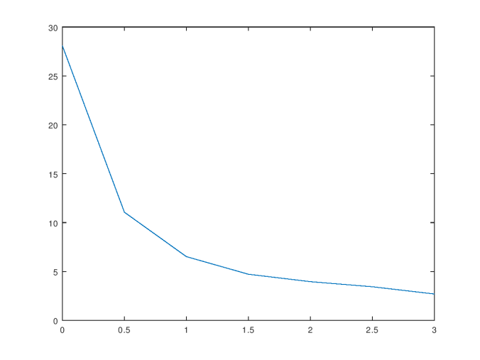
I’ve attached a color bar that begins with black (0 0 0), and increases linearly by a factor of 25.5 along the blue channel, together with a graph that shows the difference between each pair of adjacent colors, as measured by . As you can see, the colors become more similar as we traverse the color bar from left to right, despite the fact that their distances in Euclidean space are constant.

 

I’ve also attached another color bar that iterates through eight colors, but in this case, the increment moves from one channel to another, as if we were counting from 0 to 7 in binary using three bits.

The actual colors used in this case are as follows:

0 0 0
0 0 128
0 128 0
0 128 128
128 0 0
128 0 128
128 128 0
128 128 128

As you can see, yet again, the measured differences in color reflect how human beings actually perceive changes in color. Note that the greatest difference is between a non-primary blue, and primary red, which is intuitively correct both analytically (since there’s no intersection between the two colors) and visually (since there is a great deal of contrast between the two colors).

Perception and Symbolic Computation

In short, if we assume that human beings perceive colors as encoded representations of underlying physical objects, then by applying principles of information theory, we can generate equations that accurately reflect how human beings actually perceive colors. Taken as a whole, this is rather remarkable, since it suggests that the human body might, at least in some cases, operate like an efficient processor of representational information. This implies that our perceptions are the result of symbolic computations that manipulate representations, rather than one-to-one approximations of external objects. In less abstract terms, this view suggests that the way we perceive objects is more like the abstract symbolic representation of the number π , than a specific decimal approximation of the number represented by that symbol. In short, it could be that human beings not only think in terms of symbolic representations, but that we actually perceive in terms of symbolic representations. If correct, this suggests that attempts to mimic human intelligence should, at least in part, be focused on intelligent symbolic computation, and not just statistical techniques such as machine learning.

When multiple sources of information produce different, possibly even superficially conflicting probabilities for the same event, the question arises as to how those probabilities should be treated. That is, different sources, or different experimental tests, could imply different probabilities for the same event. There’s no obvious objective solution to this problem, and as a practical matter, even a crude method, such as taking a simple average of the probabilities, will probably work just fine for something like determining the probabilities of a coin toss. However, when dealing with arbitrary data, perhaps even with no prior information about the mechanics that generated the data, such an approach is likely to eliminate too much information about the structure of the data itself, generating useless answers.

Any solution to this problem is really an answer to the question of how much weight we should ascribe to each probability. That is, whatever probability we ultimately arrive at as the “correct” answer can be expressed as a linear combination of the underlying probabilities, even if that’s not how we actually arrived at the correct answer. While this might seem like a trivial statement of algebra, it offers insight into the fundamental question that underlies any solution to this problem, which is, “how much attention should I pay to this piece of information?”

Shannon Coding

In 1948, Claude Shannon showed that there was a surprising connection between probability and information. Though he was arguably only trying to construct optimally short encodings for messages, he ended up uncovering a deep, and fundamental relationship between the nature of probability and information. To establish an intuition, consider the string x = (aaab), and assume that we want to encode x as a binary string. First we need to assign a binary code to each of a and b. Since a appears more often than b, if we want to minimize the length of our encoding of x, then we should assign a shorter code to a than we do to b. For example, if we signify the end of a binary code with a 1, we could assign the code 1 to a, and 01 to b. As such, our encoding of x would be 11101, and since x contains 4 characters, the average number of bits per character in our encoding of x is 5/4. Now consider the string x = (ab). In this case, there are no opportunities for this type of compression because all characters appear an equal number of times. The same would be true of x = (abcbca), or x = (qs441z1zsq), each of which has a uniform distribution of characters. In short, we can take advantage of the statistical structure of a string, assigning longer codes to characters that appear less often, and shorter codes to characters that appear more often. If all characters appear an equal number of times, then there are no opportunities for this type of compression.

Shannon showed that, in general, we can construct an optimally short encoding, without any loss of information, if we assign a code of length log(1/p) bits to a signal that has a probability of p. That is, if the frequency of a signal from a source is p, and we want to encode that source, then we should assign a code of length log(1/p) to the signal. It follows that if a source has N possible signals, and the probability of each signal is 1/N (i.e., the signals have a uniform distribution), then the expected code length of a signal generated by the source is log(N).

Resource Management and Human Behavior

Even though it is ultimately a human being that will assign a code to a signal, and therefore ascribe information to the signal, if we take a step back, we see that, using an optimal encoding, a low probability event carries more information than a high probability event. Moreover, Shannon’s coding method is objectively optimal, in that it is not possible to construct a better encoding without losing information (if we’re considering only the distribution of the signals). That is, a source generates signals, not information, but once a human being observes a source, a representational system is required if that person wants to record, or communicate, the signals generated by that source, which will produce information. As a result, though a human being must take the active steps of observing a source, and then encoding its signals, there is an objective component to the statement that low probability events carry more information than high probability events. This is consistent with common sense, and possibly even how our brains filter information. Put crudely, as an example, high probability stories are generally considered boring (e.g., “I went to my local pub last night”), whereas extraordinary, and unlikely tales generally garner a great deal of attention and inquiry (e.g., “I met a celebrity at my local pub last night”).

You could take the view that this is just an oddity of human nature, and that people prefer unusual tales. Alternatively, you could also take the view that it is instead the consequence of something much more profound about how our brains filter out the information that constantly bombards our senses. Specifically, it seems possible that our decisions allocate resources to the experiences most likely to generate the lowest probability signals, thereby maximizing our information intake. Without spending too much time on the topic, this view could explain why human beings are generally drawn towards things and experiences that are presented as exclusive, rare, or unusual, and less enthusiastic about things and experiences that are presented as common, or mundane. In this view, pretensions and preferences are the product of a rational resource management system that allocates the senses towards experiences that are most likely to maximize the amount of information observed.

Information and Probability

Returning to the original problem above, the probability of an event should then be a function of the probabilities implied by a data set, and the importance of each data point in our data set. For simplicity, let’s assume that we have total confidence in the data from which we derive our probabilities. That is, we’re assuming our data is free from errors and reflects events that actually occurred, and were properly measured and recorded.

Let’s begin with the classic example of a coin toss, and assume that 5 people are all tossing perfectly identical coins, 25 times each, and recording the results. If one of those 5 people came back and said that they had tossed 25 heads in a row, we would probably view that as extraordinary, but possible. Considering this person’s data in isolation, the observed probability of heads would be 1, and the observed probability of tails would be 0. In contrast, our ex ante expectation, assuming the coins were expected to be a fair, would have been that the probability of each of heads and tails is 1/2. Assuming that all of the other people come back with roughly equal probabilities for heads and tales, our outlier data set would assign a probability of 1 to an event that we assumed to have a probability of 1/2, and a probability of 0 to another event that we assumed to have a probability of 1/2.

Before we consider how much weight to ascribe to this “outlier” data, let’s consider another case that will inform our method. Now assume that instead, 4 out of the 5 people report roughly equal probabilities for heads and tails, whereas one person reports back that their coin landed on its side 13 times out of 25 tosses, and that the remaining tosses we’re split roughly equally between heads and tails. That is, rather than landing on heads or tails, the coin actually landed on its side 13 times. This is an event that is generally presumed to have a probability of 0, and ignored. So upon hearing this piece of information, we would probably be astonished (recall that we are not calling the data itself into question). That is, something truly incredible has happened, since an event that has a probability of effectively zero has in fact happened 13 times. Considering the data reported by this person in isolation, we’d have an event that generally has an ex ante probability of 0 being assigned an observed probability of about 1/2, and then two events that typically have an ex ante probability of 1/2 being assigned observed probabilities of about 1/4.

Now ask yourself, which is more remarkable:

(1) the first case, where the person reported that an event with an ex ante probability of 1/2 had an observed probability of 1; or

(2) the second case, where the person reported that an event that had an ex ante probability of 0 had an observed probability of 1/2?

Though the magnitude of the difference between the ex ante probability and the observed probability is the same in both cases, the clear answer is that the second case is far more surprising. This suggests an inherent asymmetry in probabilities that are biased towards low probability events. That is, “surprisal” is not a function of just the difference between the expected probability and the observed probability, but also of the probability itself, with low probability events generating greater “surprisal”.

If we return to Shannon’s formula for the optimal code length for a signal, we see this same asymmetry, since low probability signals are assigned longer codes than high probability signals. This suggests the possibility that we can mirror surprisal in observations by weighting probabilities using the information content of the probability itself. That is, we can use the optimal code length for a signal with a given probability to inform our assessment as to how important the data underlying a particular reported probability is.

Under this view, the reports generated by the people flipping coins will contain different amounts of information. The more low probability events a given report contains, the greater the information contained in the report, implying that data that describes low probability events quite literally contains more information than data that describes high probability events. As a result, we assume that for a given event, the data underlying a low reported probability contains more information than the data underlying a high reported probability.

Information-Weighted Probabilities

Rather than simply weight the probabilities by their individual code lengths (which might work just fine in certain contexts), I’ve been making use of a slightly different technique in image recognition, which looks at how much the information associated with a given data point deviates from the average amount of information contained across all data points in the data set. Specifically, the algorithm I’ve been making use of partitions an image into equally sized regions, with the size of the region adjusted until the algorithm finds the point at which each region contains a maximally different amount of information. That is, for a given region size, the algorithm measures the average entropy of each region (by analyzing the color distribution of each region), and then calculates the standard deviation of the entropies over all regions. It keeps iterating through region sizes until it finds the size that maximizes the standard deviation of the entropies over all regions. This ends up working quite well at uncovering structure in arbitrary images with no prior information, with the theory being that if two regions within an image contain legitimately different features, then they should contain objectively different quantities of information. By maximizing the information contrast of an image, under this theory, we maximize the probability that each region contains a different feature than its neighboring regions. I then have a second algorithm that is essentially an automata “crawl” around the image and gather up similar regions (see the paper entitled, “A New Model of Artificial Intelligence” for more on this approach).

By analogy, if we have a set of probabilities, , all purportedly informing us at to the probability of the same event, then we can assign weights to each probability that reflect how “unusual” the information content of the probability itself is in the context of the other probabilities. We begin by taking the logarithm of the reciprocal of each probability, log(1/pi), which gives us the optimal code length for a signal with a probability of pi. We’re not interested in encoding anything, but instead using the code length associated with a probability to measure the information contained in the data that generated the probability in the first instance. This will produce a set of code lengths for each probability , with lower probabilities having longer code lengths than higher probabilities. We then calculate the average code length over the entire set, u. This is our average information content, from which we will determine how “unusual” a probability is, ultimately generating the weight we’ll assign to the probability. In short, if a probability was generated by an unusually large, or unusually small, amount of information relative to the average amount of information, then we’re going to assign it a larger weight.

Specifically, we calculate the weight for each probability as follows:

That is, we take the variance and add 1 to it, producing a set of weights that are greater than or equal to 1. This produces a probability given by the weighted sum,

,

where is the sum over all weights.

This formulation gives greater weight to outlier probabilities than those that are closer to the average probability, but because we begin with the code length associated with each probability, and not the probability itself, we overstate outlier low probabilities more than outlier high probabilities. That is, this method reflects our observations above, that events that have lower probabilities generate more surprisal, and therefore, “get more attention” in this method. Put differently, this method balances both (1) how “unusual” a data point is compared to the rest of the data set, and (2) how much information went into generating the data point. Since lower probability events are generated by data that contains more information (which is admittedly an assumption of this model), unusual low probabilities are given more weight than unusual high probabilities, and average probabilities have the same, minimum weight.

For example, the information weighted probability of the probabilities {.8 .8 .05} is 0.47. In contrast, the simple average of those probabilities is .55.

Note that this method doesn’t require any ex ante probabilities at all, so the question of what “prior” probability to use is moot. That is, this method takes the data as it is, with no expectations at all, and generates a probability based upon the assumed information content of the data that generated each probability. As a result, this method could be useful for situations where no prior information about the data is available, and we are forced to make sense of the data “in a vacuum”.

All,

I’ve assembled all of my additional notes on time-dilation and information theory on my blog at researchgate here:

https://www.researchgate.net/project/Information-Theory-16

I’ve also attached pdf copies of the documents here.

Regards,

Charles

A Unified Model of the Gravitational, Electrostatic, and Magnetic Forces (43)

Non-Local Interactions, Quantum Spin, the Strong and Weak Forces, and Inertia (21)

CompModofTD5-1v2 (35)

Mass_Energy_and_Momentum

MomentumMagnetismWaves25

 

On_the_Value_of_Gamma

 

Following up on previous posts (available on my research blog here) in which I presented algorithms rooted in information theory that identify structure in images, I’ve come up with a series of algorithms that together allow for very fast image categorization.

Using the algorithms presented in previous posts, the process starts with breaking an image into a set of equally sized rectangular regions. These regions are sized so as to maximize the standard deviation of the entropies of the regions. That is, we size the regions so that they contain maximally different amounts of information. This process alone uncovers quite a bit of structure within an image, and is extremely fast, generally taking only a few seconds on an ordinary laptop. See the previous posts for more on this process.

Next, the algorithm assembles these regions into larger features, using an automata that “crawls” around the image, grouping similar regions together into larger contiguous features. The question arises as to how similar two regions need to be in order to be considered part of a larger contiguous feature. Previously, I answered this question by grouping regions that are within one standard deviation of each other (as measured using a metric I describe in previous posts). This method works very well in general, and is very fast. However, it misses smaller structures in more complex images, such as busy city streets.

So instead, this set of algorithms iterates through different multiples of the standard deviation, beginning with a very small fraction of one standard deviation, and iterating up to one standard deviation. The algorithm then chooses the multiple of the standard deviation for which the structure of the features begins to “crystallize”. That is, the algorithm stops partitioning the image at the point where the structure of the resulting features is most stable. The stability of the structure of the features is tested by measuring the stability of the entropy of the distribution of the features. That is, once the distribution of the features identified by the algorithms begins to stabilize, the algorithm stops partitioning the image.

For example, if between .5*std_dev and .6*std_dev, the number and distribution of features is roughly constant, and is the most stable when compared to all other intervals, then the algorithm will choose delta = .5*std_dev as the optimal value for purposes of testing how similar neighboring regions must be in order to be grouped into a single contiguous feature.

In general, the algorithm measures the difference between H(i), the entropy of the distribution of features using a delta of (i*alpha*std_dev), and H(i+1), the entropy of the distribution of features using a delta of ((i+1)*alpha*std_dev), and chooses the value of i that minimizes,

|H(i) – H(i + 1)|.

The theory underlying this approach is that when we don’t distinguish between any of the regions within an image (by using a delta of infinity), the information content of the resultant partition (i.e., the entropy of the distribution of features) is zero, since we are in this case treating the image as one giant feature. That is, the difference between any two regions is finite using any method of comparison, and so if delta is set to infinity, all of the regions will be indistinguishable, producing one feature: the entire image. This feature appears exactly once (since it is simply the entire image), meaning H = 1*log(1) = 0.

As we begin to distinguish between regions, by using a smaller delta, we’ll end up partitioning the image into more and more features. As a result, the entropy of the distribution of features will increase (since it increases as a function of the number of features), reaching the maximum at the point where we distinguish between each region within the image, thereby maximizing the number of features. Though there could be local maxima along the way, as a general matter, the entropy of the distribution of features will increase as we reduce delta, thereby distinguishing between more and more regions within the image, generating a finer partition of the image.

There should, however, be a point along the way at which we actually uncover the “real” structure of the image, which means that the partition should be roughly stable for some interval near that point. Put loosely, the real structure of the image should be “in focus” within some small window around the objectively correct partition.

These algorithms attempt to find that correct partition by choosing the value of delta for which the derivative of the entropy of the distribution of features, as a function of delta, is minimized. This is the point at which the structure of the features, and the number of the features, changes the least as we alter delta, and where we assume the structure of the image is most likely to be “in focus”.

I have attached examples showing the structure identified by these algorithms. The images attached to this post have been weighted by their S-score, so that the most notable features are the brightest, and the least notable the darkest. The S-score is, in short, a measure of how notable a region is in terms of its information content. The shading here “paints” a feature according to the average S-score over all regions within the feature.

Finally, once all of that pre-processing is sorted, another algorithm goes through the features that have been identified in one image, and compares them to the features identified in another, by using six statistical properties of the features, each of which are invariant under rotation:

(1) The partition score N, which is the point at which the “information contrast” of the feature is maximized. See previous posts for more on this.

(2) The standard deviation of the entropy of the feature, as calculated using the partition score N. This is a measure of how much variation there is in the statistical color structure of the feature. A “boring” feature will have a low score, and a “complex” feature that changes color distributions often will have a high score.

(3) The average entropy of the feature, as calculated using the partition score N. This is a measure of how evenly distributed the color information is, with features that have a very concentrated color distribution scoring low, and features that have a very wide distribution of colors scoring high.

(4) (5) and (6) are the average colors across the R,G, and B channels of the feature. This is used to capture the “actual” average color of the feature.

The norm of the difference of the resultant 6-vector for the two regions being compared is then calculated, and averaged over all features, weighted by the importance of the region, as measured using the “S-score” I presented in previous posts. The larger the resultant score, the less similar the two images are. Categorization can then be achieved by comparing the scores generated when one image is compared to a series of images from two or more different categories, allowing us to predict to which category the input image most likely belongs.

Pre-processing an image using the attached algorithms takes anywhere between a few seconds and a few minutes (on a very low-fi laptop), depending upon the size of the image, and its complexity.

Comparing two pre-processed images takes fractions of a second, making processing time for comparing pre-processed images generally negligible. This suggests that these algorithms would likely be able to process video in real, or close to real-time, on an industrial machine. This would allow, for example, live video to be compared to pre-processed databases of images, in order to determine the most likely subject matter of the features within the video.

The code should be called from the Octave command line as follows:

I = imread(“[FILE PATH]”);
[region_matrix N S_mat feature_score_vector] = identify_features(I);
imshow(ent_contrast_darken(I,N,region_matrix, S_mat));

To compare two images that have been processed, use the following:

average_score = IMG_Comparison(region_matrix_1, N_1, S_mat_1, feature_score_vector_1, region_matrix_2, N_2, S_mat_2, feature_score_vector_2)

Octave Scripts

ent_contrast_darken

extract_region

gather_regions_delta

generate_weight_matrix

identify_features

IMG_Comparison

local_test

Attached is code that I wrote in Octave that can, without any training data or other prior information, identify features within an image. It is a completely deterministic algorithm that does not make use of any statistical, or machine learning techniques.

The theoretical basis of the algorithm is that objectively distinct features of an image should contain different amounts of information. The algorithm measures information content using the Shannon Entropy of the color distribution of the image. Specifically, it breaks an image into a series of sub-images, and then measures the Shannon Entropy of those sub-images.

It begins by measuring the entropy of the image as a whole, and then divides the image into equally sized regions of 4, 9, 16, … N^2 sub-images. It then calculates the entropy of each region, for each value of N. It then selects the value of N that maximizes the standard deviation of the entropies of the regions.

The theoretical significance of this maximization is that the image is, as a result, broken into sub-images that contain maximally different amounts of information, which we view as a proxy for regions that contain objectively distinct physical features.

Using the optimal value of N generated as described above, we then weight the pixel values of each of the resulting N^2 regions by,

S = (Hu – HR)^2/s^2

where Hu is the average entropy over all regions of the image, HR is the entropy of the region in question, and s is the standard deviation of the entropies over all regions within the image. That is, if a region contains an amount of information that is approximately equal to the average amount of information contained across all regions of the image, it will be darkened significantly; whereas if a region contains an amount of information that is significantly above or below average, it will be brightened significantly.

The net result is (1) “unremarkable” regions are significantly darker and “notable” regions are significantly brighter, and (2) the image is “quantized” into regions.

I have attached two examples of images that were processed using this algorithm. One is of myself on a boat, in which the algorithm clearly recognizes my eyes, mouth, ears, and hand (and my beer). The other is of handwritten text (which was not subject to copyright), and it clearly recognizes the portion of the page with text, and the pen. As noted above, the algorithm is not trained to notice anything at all, and is entirely deterministic.

It turns out that the algorithm is actually quite good at pulling features from all types of images, regardless of subject matter.

I have also attached a “fast” algorithm that searches for an optimal value of N, rather than simply iterating through all N (attached as “maximize_std_dev”, an outline of which is also attached as a handwritten note that is easier to follow).

The functions should be called from the Octave command line as follows:

I = imread(” [ Image file path ] “);
[N Y X] = maximize_std_dev(I);
Z = ent_contrast(I,N,X,Y);
imshow(Z);

Z will contain the entropy-adjusted image. The original image must be in an RGB format.
I’ve also attached two scripts that compare two images using this approach, and return a score that measures how similar they are (Delta), after their features have been extracted. The comparison algorithm attached is set up to compare two individual images, but is really intended to compare one image to two databases of images.

For example, in the spirit of Google’s “bird vs bike” contest, this algorithm is intended to take an input image, and then compare it to a database of bird images, and a database of bike images. Which ever database generates the greatest average score per image within the database is the “most similar” to the input image.

The algorithm works by comparing the average color and the standard deviation of the color of each region of both images generated using the algorithm above. That measure for each region is then weighted according to the product of (X) the information contained in that region, as measured using its entropy, and (Y) the “importance” of the region, as measured by S above. The theory behind the algorithm, is that the more information a region contains, the more “points” the algorithm should allocate for each “unit” of similarity; and the more “important” a region is, as measured by S, the more “points” the region should get for each “unit” of similarity.

Interestingly, because the algorithm does not make use of any “real” shape information, it is invariant under rotation. Nonetheless, it seems to work quite well.

The functions should be called from the command line as follows, after the images I1 and I2 have been processed using the algorithm described above:

[A1 B1 C1 D1] = score_image(I1,N1,X1,Y1);
[A2 B2 C2 D2] = score_image(I2,N2,X2,Y2);
temp = size(I1);
num_pix_1 = floor(temp(1)/N1)*floor(temp(2)/N1);
temp = size(I2);
num_pix_2 = floor(temp(1)/N2)*floor(temp(2)/N2);
Delta = weighted_img_compare(A1,B1,C1,D1,N1,Y1,num_pix_1,A2,B2,C2,D2,N2,Y2,num_pix_2)

Finally, note that the Octave “image” package is required to run this algorithm.

 

Octave Scripts:

weighted_image_compare

test_measures

score_image

MaximizeSTDDEV-Summary

maximize_std_dev

ent_contrast

 

Globalization has dramatically improved standards of living for entire populations in both developed and developing economies alike. Complex goods like laptops and smartphones can now be produced at incredibly cheap prices, allowing ordinary people to keep in touch, enjoy both traditional and new forms of media, and make payments quickly, safely, and easily. These communication networks and devices are not only beneficial to human welfare, but are also a tremendous achievement for humanity as a general matter, and mark the first steps towards a single, truly integrated global economy.

But globalization has also altered the fundamental balance of power between labor and capital. One of the most alarming consequences of this new balance of power is the growing divide between the incomes of the professional class and the working class, and the even larger divide between the incomes of the investor class and everyone else. Though economies are complex systems, the fundamental cause of these income gaps can be traced to the relatively lower price of labor in many of the markets where these goods and services are now sourced, as compared to the price of labor in developed economies. Unfortunately, this relatively lower price of labor is in many cases due to the local absence of social and political institutions necessary to protect people from being exploited, meaning that human beings can in some markets be forced to work for little or no compensation, often in unsanitary, and unsafe conditions. At the same time, global supply chains have grown to be so complex, that even well-intentioned corporations have to dedicate significant resources to ensure that their products are produced without the use of exploitative labor, or at a minimum, to ensure that their supply chain is in compliance with modern anti-slavery laws.

Though there was some outrage over the Libyan slave auctions that made it to the headlines in 2017, consumers seem generally oblivious to the fact that in 2018, millions of people are being forced to work for little or no compensation. The International Labor Organization estimates that on any given day during 2016, there were 40.3 million people globally that were used as slaves.

Slavery is now, without question, an integral part of the modern global economy.

The Single Market

Globalization is gradually creating a single, global market for goods and services. As the market for labor became globalized, the effective supply of labor increased, causing the price of low-skill labor to generally decline in developed economies (see page 25), eventually causing the income generated by capital to come very close to parity with the income generated by labor in developed economies. This means that, as a class, the developed world’s investors and property owners now generate almost as much income from their capital as working people generate through their labor. Similarly, financial markets have become increasingly correlated globally, as capital is now generally free to move across borders, and global investors concentrate their capital with a relatively small number of large, global asset managers.

The power gap between the global investor class and the working class in developing economies is even more pronounced. Historically, many developing economies have contributed only marginally to the overall global economy. As a result, many governments in developing economies lack the political and social institutions necessary to protect their populations from being exploited by foreign capital, particularly in rural areas, where children have little to no access to formal education (see pages 20 to 21).

As markets became more integrated over the last thirty years, small, developing economies began to contribute meaningfully to the global economy, in turn attracting significant investments from large corporations and wealthy individuals alike. This has of course created wonderful opportunities for many people in developing economies, and lifted entire populations out of poverty in China, India, Brazil, and elsewhere. But at the same time, the lack of political and social institutions in many developing economies has created an environment where human trafficking, exploitative labor, and even outright slavery are occurring on a mass scale.

While these may sound like marginal, outlier cases, it is important to remember how large the world’s population is right now: approximately 7.6 billion people. This means that bad outcomes with low probabilities still involve millions of people being harmed. Left unchecked, this dynamic will inevitably lead to a shift in normative expectations and behaviors, where consumers and businesses alike grow accustomed to the idea that some amount of abusive or exploitative labor is inherent in the production of a modern product, simply because production is now so complex, that it is impossible to sift through the entire supply chain and uncover all the bad actors. In economic terms, just as the price of labor appears to be converging to a global average, the culture of labor could also converge to a global average, as the consumer class collectively grows indifferent to how the products and services they use are being produced.

By analogy to the financial markets, when credit markets heat up, the price of borrowing comes down, meaning that borrowers pay lower interest rates on their loans as lenders compete with each other. But something else tends to happen under these conditions: the terms of the loan documents become more favorable to the borrower, as lenders find other, softer ways to compete with each other, beyond pricing. Similarly, states that all have a comparable cost of labor will find other, “softer” ways of competing with each other, beyond the price of labor. In developed economies, states might compete with tax incentives, or regulatory exemptions. For example, individual states within the U.S. are now in the process of competing for Amazon’s new headquarters, since Amazon’s new home state will almost certainly benefit from a large investment by the company, leading to new jobs, infrastructure development, and tax revenues. This creates an incentive on the part of elected representatives to offer terms beyond the price of local labor that Amazon will find attractive. In developing economies, or in resource rich, but otherwise impoverished economies, the process of courting capital by state officials lacks the oversight and legal roadblocks that developed economies have put in place over hundreds of years of commerce and investment. This results in an environment where bribery and corruption are viewed as standard practices in many markets.

Globalization has of course also given rise to global corporations, meaning that local corruption is no longer a local problem, as large, global brands do business with small, often corrupt local regimes, whether directly, or indirectly through their supply chains, or other business relationships. This again runs the risk of a type of normative averaging, where global businesses become desensitized to corruption, bribery, and abuse, whether through their own direct contact with corrupt businesses, regimes, and individuals, or through the awareness of more attenuated relationships.

One of the benefits of a free market economy is that there is no single, conscious architect of its outcomes, which means that complex economic decisions are determined by the wisdom of crowds, through the idiosyncratic preferences and decisions of a growing population of billions of individuals acting without any collective plan. In contrast, the management of capital has become more and more concentrated into a relatively small number of similarly minded firms and individuals, giving these firms and individuals significant control over the world’s publicly traded companies, and private companies (see page 15). As the income generated by capital inches closer to parity with the income generated by labor, the net effect is that billions of uncoordinated individuals will be seeking employment either directly at an asset management company, or indirectly through a company controlled by an asset management company, ultimately financed by a global investor class that has a collective income that is comparable to the total income generated by these masses, but much greater, and more coordinated, economic power.

The Decline of the Regulatory State

Bernie Madoff is a truly shameless man, whose life story is, nonetheless, in some sense, the archetypal American success story. He grew up in Queens, New York, in a working class family, went to a public high school, graduated from college, all the while without achieving any notable academic distinctions, and started what was, in fairness to him, a successful and innovative financial services firm. He eventually scrambled all the way up from the hinterlands of the pink sheets, to the Chairman’s office of the Nasdaq exchange, becoming a very rich man along the way. But Madoff’s appointment as Chairman meant more than just additional compensation and prestige for Madoff as a businessman. The appointment made Madoff a fiduciary of society as a whole. Nasdaq’s exchanges are not ordinary businesses, but are instead vital pieces of financial infrastructure, akin to public utilities: nearly $100 billion (USD) worth of transactions occur every day on Nasdaq exchanges. Madoff’s appointment as Nasdaq’s Chairman meant that he had been entrusted with one of the most important pieces of machinery in the global economy: a tool that, if misused, could easily harm millions, and possibly billions, of human beings. More worrisome, Nasdaq is a self-regulatory organization, meaning that, in practical terms, Nasdaq itself as an institution can write and enforce many of the regulations that govern the conduct of the individuals that make use of its exchanges. Putting all of this in context, Madoff’s appointment as Chairman of Nasdaq borders on the comical, given that he is, of course, now known to be one of history’s greatest financial criminals.

The stark contrast between the responsibilities of Bernie Madoff’s role as Chairman, and the gross deficiency of his character, is itself evidence of regulatory dysfunction. In a well-functioning regulatory environment, an outcome where such a reprehensible man is given such enormous responsibility should have a near-zero probability of occurring. We could of course argue that, with time, even low probability events must eventually occur, and so, perhaps Madoff’s chairmanship was an outlier event that is not really evidence of anything other than a slippery man that weaseled his way to the heights of his industry. Unfortunately, this cannot be the case, as the Securities and Exchange Commission, who is ultimately responsible for Nasdaq, was warned that Madoff was likely engaging in financial crimes. This warning, together with the scale, and brazen nature of Madoff’s crimes, make it impossible to conclude that the regulatory environment in which Madoff operated was functioning properly.

The financial crisis of 2007-2008 is further evidence of a broken and dysfunctional regulatory state. While there was no shortage of discussion on the “complex” products that banks were using to “place bets” on the U.S. housing market, the reality is that mortgage-backed securities (the assets at the heart of the financial crisis) have been in use since the 1970’s in the U.S. They are of course unfamiliar to most people, but this is no different than the generally arcane products that allow any industry to function. Most people have no idea how an airplane engine works, yet people fly every day. Similarly, most people have absolutely no idea what happens at a typical bank, yet they make use of banking services every day.

When a plane crashes, the public wants to be reassured that there is nothing wrong with planes generally, but that there was something wrong with the particular plane that crashed, or the particular pilot that caused the plane to crash. If such a narrative didn’t exist, the economy would likely be crippled, as people would no longer trust aviation as a safe means to transport human beings and goods. Similarly, the financial crisis created demand for a narrative that would allow society and regulators alike to blame particular firms, individuals, circumstances, and products, so that society could get back to using banks without having any idea as to how they actually function. Such a narrative is to some degree necessary, because banks need to be able to function, whether or not people understand how they work, and ordinary, everyday people need to be able to trust the financial system with their paychecks and savings – the very means by which they feed, clothe, and house themselves and their families.

Whether we can trust our banking system, and our financial system generally, is in part dependent upon our confidence in banking and securities market regulators. Unlike individuals that have jobs at private firms, regulators are paid to act in the interests of society as a whole, and to put their own personal, economic interests aside. Of course, regulators are human beings, with all the psychological, moral, and intellectual shortcomings that are characteristic of our species. And so it would be not only foolish, but also unfair to expect regulators to conduct themselves in some sort of saintly manner that is in its nature different from that of an ordinary person. But having low expectations doesn’t imply that we shouldn’t design regulatory environments with the worst of humanity in mind. In fact, it implies that we should have laws in place that prevent regulators from acting on their worst instincts, or in a manner that creates public harm, in exchange for private benefit.

The scale of the financial crisis, and the fact that, again, regulators had reason to suspect something was wrong, together with the fact that many market participants saw the crisis coming and profited from it, suggest quite plainly that the U.S. regulatory system is broken. The narrative that was weaved after the financial crisis was that prior banking and securities laws were inadequate, and that the financial reforms that have taken place since then have addressed these inadequacies. From this we are to conclude that a new financial crisis is unlikely, since regulators are now equipped with the tools necessary to stop such an event from occurring again. This narrative, however, assumes that the inadequate regulations were in fact the sole cause of the financial crisis, when in fact the crisis was at least in part due to a much more mundane cause – banks were financing long term, illiquid assets with short term capital. When that short term capital dried up, banks had to scramble to raise capital, and some of them didn’t survive that process. This narrative also assumes that regulators will actually make use of these new tools in order to stop another financial crisis from occurring, which is obviously a very cynical line of reasoning, but the reality is that regulators, like all other rational human beings, are, generally speaking, primarily concerned with their own careers and their own lives. As a result, it is not necessary for regulators to be corrupt, in the classic, criminal sense of the word, to produce bad outcomes, but rather, to simply, whenever it is legally possible, maximize their own private benefit, possibly at the expense of the public good.

It is an open secret that there is a revolving door between financial regulators and financial institutions. And again, this does not imply that the individuals that make the skip from regulator to financier are engaging in anything that rises to the level of criminal behavior. More likely, they are simply looking out for each other in a manner that maximizes private gain, possibly at the expense of the public good. In fact, such an environment doesn’t even require deliberate, coordinated action in order for a tragedy to occur. If a sufficient number of regulators are acting in their own self interest, or ignoring, or simply not caring about their jobs, it creates a regulatory environment where regulatory diligence is low, and the probability of a financial crime, or financial crisis, is therefore high.

For those regulators that do take their jobs seriously, of which there are undoubtedly many, the prospect of regulating a global corporation must be unnerving. In 2015, Apple’s annual revenue was approximately $234 billion (USD). Though not entirely analogous, for context, the gross domestic product of Finland for 2015 was approximately $232 billion. This means that, in practical terms, the revenue raising power of Apple Inc. is on par with that of a highly developed, sovereign European state. Finland is of course a small country compared to the United States, but it is nonetheless a first-rate nation with a high-functioning government, education system, infrastructure, and military. All of these institutions within Finland are beholden to the people of Finland, and operate for the benefit of the people of Finland. In contrast, Apple Inc. is a corporation that operates for the benefit of its global shareholders, who have no obvious, collective interest other than making a profit. Apple Inc. is in this sense an extremely wealthy state without a land, a people, a parliament, or a purpose, beholden only to what is shaping up to be a single class of global investors.

Apple is of course not alone, and is instead but one example of a modern, global corporation that has all the money and power of a sovereign state, but none of the obligations or cultural history of a sovereign state. The world’s largest financial institutions are of course comparable in scale, complexity, and power, but they are, in contrast to Apple, much older institutions, with deep, historical ties to governments all over the world. This makes the task of regulating a financial institution a precarious one for the individual human beings employed by financial regulators. Imagine working as a government regulator, and having the nerve to tell another person that works for a giant financial institution (who in a few years could very well be your boss, or alternatively, offer you a high-paying job) with tens, or even hundreds of thousands of employees, and the financial resources of an E.U. member state, that they need to change their behavior: this is not going to be the average case. So as a practical matter, the power imbalance between individual regulators and the institutions they regulate instead ensures that individual regulators will be cautious in their interactions with management-level contacts at the institutions they regulate, and only go for blood when instructed to do so by their superiors.

Common sense suggests that such an environment will inevitably lead to bad outcomes, and recent history is, not surprisingly, in agreement with common sense. But instead of questioning the obvious problems created by the incentive and power structure of the current regulatory environment, and the power imbalance between individual regulators and the massive, global corporations they oversee, lawmakers and enforcement agencies tend to focus on headline grabbing cases, emphasizing outrage, and short-term justice, rather than making sensible, substantive reforms. Frankly, this is all done to create the appearance of a well-functioning regulatory state, and to distract from its glaring, and destabilizing shortcomings. Lesser known corners of the U.S. financial system, such as underfunded state and local pension plans, get almost no popular attention at all, and arguably lack a competent regulator in the first instance. Yet, they could pose serious risks for the financial markets as demographics shift, causing pension liabilities to become due to beneficiaries.

This is not to say that the post-crisis financial reforms were superficial in nature. To the contrary, the reforms brought about by the Obama administration were vast in scale, very expensive to implement, and fundamentally changed many business lines at financial institutions, and the financial market’s structure generally. But the fundamental relationship between financial regulators and financial services firms remains generally unchanged, and as a result, incumbent firms will likely continue to operate with effective impunity, while occasionally, individual actors will of course, probably be punished, and made an example of, in order to create the superficial appearance of justice, when in reality, a regulatory system that functions properly should never produce these types of outcomes in the first instance.

Though there is unfortunately no shortage of examples, Bernie Madoff is the archetypal case of the dysfunction of the U.S. regulatory and justice system: rather than stop his criminal conduct from occurring in the first instance, or prevent it from reaching a dangerous scale, he was instead arrested and convicted after the fact, and sentenced to 150 years in prison. These types of sentences, that pointlessly run longer than any human lifetime, especially for an already old man, say a lot about how justice now works in America. It’s not a justice system that actually prevents bad outcomes, but is instead a justice system that gives us something to marvel at, and talk about, after the harm has already been done – the scale of Madoff’s crime, his outrageous lifestyle, all culminating in a bizarre, and meaninglessly long jail sentence. The U.S. justice system is, as a general matter, now rooted in spectacle, not substance, and the results reflect this.

The Rise of Criminal Business Conduct

The Grey Market

People that are not themselves criminals generally have a very romanticized notion of what it is to be a criminal. This is only natural, since if you are not a criminal, you probably don’t interact with criminals on a regular basis, and so you’ll fill in the mental gaps as to how criminals behave with bits gleaned from movies, novels, and documentaries, all produced by people that are probably not criminals themselves. As a result, people that grow up with light bulbs, bank accounts, and clean underwear, are in this sense detached from what ordinary life is like for people that have to use violence to survive on a daily basis. All of this produces a mental portrait of criminality collectively painted by a group of people that are generally out of touch with how remarkably disgusting, and incredibly brazen, criminally minded human beings can be.

Prior to the integration of the global economy, this criminal knowledge gap didn’t really matter much, since criminal conduct was largely a local issue, dealt with by local authorities who were experts in the behavior of local criminals. But just as globalization broke the shackles of geography for businesses, spawning the birth of giant, global corporations, globalization has also knocked down the gates for criminal enterprises as well, allowing intrepid, criminally minded individuals and organizations to conduct business on an unprecedented, global scale. And because otherwise legitimate global firms now interact with small, often corrupt local regimes, there are likely more interactions taking place between large global institutions, and quasi-criminal organizations and corrupt state actors, blurring the lines between commercial and criminal conduct. As a general matter, this means that local corruption is, again, a global problem.

There are some astonishing recent examples of this “grey market” for goods and services, where otherwise legitimate firms and individuals engage the services of others that perform deliberately criminal, or potentially criminal acts on their behalf.  For example, Harvey Weinstein apparently hired former Mossad agents to bully women he had abused in an effort to cover up his criminal sexual conduct. Save for his sex life, Harvey Weinstein does not appear to have been otherwise engaged in a criminal enterprise, but he was nonetheless able to find, and pay, others to perform potentially criminal acts act on his behalf.

Bloomberg recently published an in-depth piece about the mystery of an oil tanker that was hijacked under suspicious circumstances while carrying $100 million (USD) worth of oil. The investigation that followed, carried out by the company that provided the insurance for the ship, spurred what appears to have been a dramatic assassination of the insurance inspector: one day after the insurance inspector reported back that the hijacking did not appear to have been carried out by ordinary pirates, a bomb went off in his car, killing him instantly.

For the all the purported rough and tumble of Wall Street during the 1980s, the “barbarians at the gate” probably didn’t deal with car bombs, or Mossad agents, so it seems that being an insurance inspector or an actress in 2018 requires more grit than being a private equity titan did in the 1980’s.

There are also cases of criminals infiltrating legitimate businesses in order to use them for criminal ends. In an age where people’s personal information (text messages, photos, internet history, etc.) can all be used to blackmail them, otherwise ordinary people with access to sensitive information, or a particular set of skills, could find themselves under the thumb of organized crime. Bloomberg ran yet another in-depth piece about how two Belgian IT consultants, both earning six-figure salaries in their professional careers, ended up being coerced into working with Turkish mobsters, using their IT skills to steal access codes to shipping ports, ultimately to facilitate the smuggling of cocaine and heroin on a mass scale.

Similarly, financial institutions can be used by economically or politically motivated individuals willing to commit financial crimes, whether for a profit, or to advance a political agenda. The complexity and scale of financial institutions, and the global financial markets generally, allow connections between otherwise legitimate firms and criminal organizations, or rogue states, to go undetected through obfuscation. Financial institutions that facilitate money laundering, or transactions that run afoul of sanctions, in this manner can do mass harm, funneling enormous sums of money to dangerous individuals, and undermining the effect that sanctions are intended to have on the states and individuals they are intended to punish.

Donald Trump’s Business Network and Political Campaign

For all his anti-globalist rhetoric, Donald Trump is in reality a globalist businessman. His real estate, entertainment, and other businesses are all part of a sprawling global network of companies that have benefited from the same low barriers to trade that he is now putting in the cross-hairs. Though Trump has made good on his campaign promises, and has begun to impose trade tariffs, he is conspicuously silent on the tremendous sums of money that cross international borders every day through the global financial system.

According to several reports by the Financial Times, it now seems that Trump has personally benefited significantly from the types of grey market transactions that have been facilitated by the emergence of a global, decentralized financial system that lacks a single, competent, global regulator. As if taken from the pages of a poorly written screenplay, the sordid list of characters involved in Trump’s extended business network includes the KGB itself, shady Canadian real estate developers, thugs (including Felix Sater, who served time in prison for stabbing an associate in the face), and of course, porn stars. Despite the scale, and to his credit, the generally public, and often ostentatious, nature of Trump’s businesses, no competent regulator thought it necessary to stop Trump’s financial dealings before they occurred.

Similarly, no competent regulator was able to identify and stop the proliferation of political disinformation on Facebook that occurred during the 2016 elections, which increasingly appears to have been done at the direction of the Russian state. That Facebook could be used as a tool to alter election outcomes seems obvious in retrospect, since it is a source of news and information for billions of people. That Facebook could be exploited by foreign or domestic groups looking to deliberately alter election outcomes also seems obvious in retrospect. Yet, there is no single, competent regulator for a company like Facebook, despite its power to influence the thoughts and opinions of billions of people globally. You could of course argue that Facebook’s power to shape the thoughts and opinions of its users is speculative, but this is nonsense: businesses and political campaigns alike pay Facebook billions of dollars in ad revenues precisely because Facebook can, by exploiting the vast body of sensitive, personal information it has on its users, change the way people think about products, services, other people, and issues.

The Dark Web

The same communication and payment infrastructure that facilitated the rise of global trade also gave rise to a decentralized, generally anonymous communication and payment network loosely referred to as the “Dark Web”. Intelligence agencies, criminals, and increasingly, children without direct access to the black market, all use services like Tor to communicate and transact with each other over the Dark Web, on a global, generally anonymous basis. The Dark Web has commoditized the black market, removing many, and in some cases nearly all, of the logistical barriers to purchasing drugs, guns, sensitive information, and even human slaves.

Though law enforcement agencies are certainly aware of the Dark Web, it is a global, and decentralized network of servers and individuals, and as a result, there is no obvious law enforcement, legislative, or regulatory solution to the criminal conduct taking place on the Dark Web. Global law enforcement officers have, however, made significant busts, including the break up of Silk Road, and a recent bust involving the FBI and Europol, in which two Dark Web sites dealing primarily in drugs, weapons, and malware were taken down. One of the sites, AlphaBay, reportedly could have had annual revenues of several hundred million dollars. Despite these potentially large revenues, the AlphaBay case resulted in only a few arrests, since the individuals who were apparently running the site were few in number, and scattered all over the world.

Like a leanly staffed tech startup, or hedge fund, global communications and payment networks like the Dark Web allow a handful of ambitious criminals in disparate locations to conspire, and generate enormous sums of money, something that likely would have been impossible only twenty years ago. In contrast, a law enforcement operation to break up an enterprise like AlphaBay requires high-level coordination between multiple law enforcement organizations across different international jurisdictions, all running up hill, trying to identify a small number of individuals who all go through great efforts to remain anonymous. In simple terms, it is much easier and cheaper for a small number of criminals to set up something like AlphaBay, than it is for global law enforcement agencies to tear it down. This means that the moment a site like AlphaBay is taken down, competitors will likely pop up to fill the void, which is apparently exactly what happened.

There are the classic black market items for sale on the Dark Web, such as drugs, guns, and child pornography, but the flexibility and anonymity of the dark web has also created a forum for transactions in new forms of contraband, such as sensitive personal information, classified or otherwise sensitive government documents, and human beings. In the summer of 2017, a twenty year old British woman was kidnapped and drugged while on vacation in Milan, and auctioned off, presumably as a slave, on the dark web. The group that perpetrated the kidnapping, “Black Death”, was known to the media since at least 2015, but some sources believed at the time that Black Death was a hoax. Two years later, it became clear that Black Death is not only an unfortunate reality, but that it is entirely possible that there are scores of other less fortunate victims of human trafficking facilitated by the Dark Web that have gotten no attention at all from law enforcement, or the press.

The Rise of the Global Far-Right

The quality of Trump’s relationship with a foreign leader seems to turn on whether or not that leader can be characterized as far-right. Vladimir Putin, Kim Jong-un, Recep Erdoğan, and Rodrigo Duterte all seem to score high marks from Trump. In contrast, Trump is hostile toward democratic leaders such as Angela Merkel, Emmanuel Macron, and Theresa May. Though his relationship with China is generally adversarial, his initial relationship with Kim Jung-un also began on very shaky grounds, yet ended in bromance. So perhaps this is merely the opening act of what will eventually turn into a courtship dance between Trump and Xi Jinping. Trump’s reaffirmation of the U.S.’s commitment to Israel comes at a strange time for the state of Israel and its people, as Israel has itself been increasingly welcoming of far-right, Eastern European politicians.

Though the history has long left the headlines, the Italian far-right was believed to be behind much of the terrorism that took place there during the 1980’s. Behind Italy’s far right, however, were criminal and quasi-criminal organizations, such as Propaganda Due, who sought to use the resultant political upheaval and popular outrage to launch the political careers of their own members, including Silvio Berlusconi. In the end, while these groups may very well have had a political vision (they were purportedly fascist, anti-communists), the means by which they achieved their ends was to foment political discord using terrorism, and then offer up their own members as political candidates to “solve” the very problems they had created in the first instance.

On the economic front, these groups made use of a sophisticated mix of corporate takeovers, financial crimes, and brutality to secure control of major corporations across Europe. (“God’s Bankers” is a thoroughly researched, nearly scholarly work, on the history of the Vatican Bank, which includes a detailed history of the rise of Propaganda Due). The end result is that a small number of criminal and quasi-criminal actors with deep ties to the Italian state, Italian intelligence, and the Vatican Bank, ended up controlling significant swathes of the Italian economy, and political system, causing several financial disasters along the way, including the collapse of an American bank, the Franklin National Bank. This brand of high-level, highly-organized crime has almost certainly contributed to the present Italian state, which is notorious for crippling dysfunction, corruption, and a preposterous justice system – all of which can now fairly be said of the U.S. government.

Taking the rise of Propaganda Due in Italy as a case study, it is entirely possible that the hands behind the current, global rise of the far right have no genuine political motivation whatsoever, but are instead primarily economic actors, interested only in dysfunctional, weak political states. Weak states, whether through outright corruption, or indifference, allow quasi-criminal organizations like Propaganda Due to carry on with lower boundaries to action. These “men of action”, as the members of Propaganda Due refer to each other, find unfettered commercial environments more conducive to their style of doing business.

You don’t need a tinfoil hat to argue that something similar has been gradually taking place in the U.S over the last thirty years. In this view, Trump’s improbable presidential victory is the climax of a slow-growing economic and political infection, brought about by unchecked flows of international capital, regulatory indifference, and the rise of corruption globally, all of which have now set in motion the possible collapse of the post war world order, and the rise of what is shaping up to be a new world order in which a handful of strongmen dominate the headlines, spending little time on substance, and lots of time massaging each other’s egos.

There is a lot of discussion as to who is responsible for all of this, and it is of course entirely possible that no one is responsible, and that the rise of the global far-right is simply the product of uncoordinated demographic, political, and economic forces. Nonetheless, the obvious culprit is the Russian state: they have both the means and the motive, as the far-right candidates that have popped up in the U.S. and Europe are universally anti-globalist, protectionists, creating the risk of a power vacuum if western democracies truly abandon the current world order, which Russia, and possibly China, would be happy to fill. But it is looking increasingly likely that if the Russians are responsible, then they didn’t act alone, and instead had the help of far-right extremists, globally. This is not to say that the same individuals that were responsible for the rise of the present Italian mafia-state are also responsible for the rise of Donald Trump. That said, Donald Trump and Silvio Berlusconi are, coincidentally, remarkably similar people: both had careers in the media prior to public office; both have rather unabashed ties to organized crime; both have been involved in sex scandals; and, bizarrely, both have signature, rather unusual tans.

Recent events suggest that there is at least superficial evidence of a connection between the far-right in the U.S., and the Russian state. And there is an obvious connection between the far-right, and gun violence, police brutality, and hate crimes, all of which are politically toxic subjects, that are undermining the effectiveness of politicians on both sides of the political spectrum, as voters become increasingly entrenched, focusing on polarizing, hot-button issues, rather than the comparatively boring, but equally important issues of financial regulation, education, trade policy, and the economic and fiscal soundness of the U.S. generally.

If the rise of the global far-right is deliberate, perhaps as designed by the Russian state to expand the sphere of Russian influence further into continental Europe, and beyond, then the same strategy employed by Propaganda Due in Italy during the 1980’s and 1990’s could be being employed in the U.S., and in western democracies generally: foment political dysfunction on both sides of the political spectrum, for example, by sponsoring terrorist activities, and in general by inciting violence (e.g., Donald Trump’s thinly veiled endorsement of police brutality), in order to poison the well of political discourse, destroy the current political order, and eventually, run an outsider candidate, like Trump, as the “solution” to those very problems.

Global trade is old — really, really old. But something new is happening to the world economy as software and container trade shrink the globe — the rate of “globalization” is increasing, allowing developing countries to hitch a ride on the capital of advanced economies and race forward.

But how do you measure how fast the world economy has “globalized” in one figure? Perhaps, by borrowing a concept originally developed by physicists known as entropy.

The mysterious and growing divide between the rich and the rest in just about every wealthy country on Earth, including the U.S., is really two mysteries wrapped in one. The first mystery is why real wage growth has sped up at the top and slowed down for everybody else. But the second, more recent, and more fascinating problem is why labor’s share of the winnings in developed economies has been in decline. It’s not just that middle-class wages are falling behind the rich. Overall wages are falling behind something else — capital.

People are becoming less valuable to companies. Why?

Continue reading on The Atlantic…