In this note, I’m going to present an algorithm that can, without any prior information, take a scrambled image, and reassemble it to its original state. In short, it shows that even if we know nothing about a distorted image, we can still figure out what the image was supposed to look like using information theory. The only input to the algorithm is data derived from the scrambled image itself, and the algorithm isn’t recognizing objects. It is instead, rearranging the scrambled image in a manner intended to maximize the expectation that any objects in the image will be reassembled.


Human beings can solve these types of puzzles easily because we have experience with real world objects, and know, whether consciously or not, what things should look like, generally. Because this algorithm operates with no prior information at all, it suggests that our intuitions for structure might have an even more primordial origin that goes beyond experience, and is instead rooted in how objects in the natural world are generally organized.
This algorithm is yet another example of the utility of my approach to artificial intelligence, which is to make theoretical assumptions based upon information theory about what should happen given a particular input, and proceed mechanistically without a dataset, with the expectation that what is generated should be useful and accurate. Interestingly, this particular algorithm can be fairly characterized as a matrix algebra algorithm, since it swaps entries in a matrix according to a simple closed form formula. As a result, this algorithm has more in common with Gaussian Elimination than a typical machine learning algorithm.
In this note, I’m going to apply this algorithm only to images, but I suspect it has more general applications in information recovery. In particular, I think this algorithm could be used to reassemble not only images, but 3D objects, and though not an area of my personal interest, it seems like it could also have applications in code-breaking and DNA analysis.
Partitioning an Image
Previously, I’ve discussed my image partition algorithm, which makes use of assumptions based in information theory in order to partition an image into objectively distinct features, without any prior information (i.e., without a dataset). You can read about this algorithm, and others, in my working paper, “A New Model of Artificial Intelligence“.
In short, the image partition algorithm breaks an image into regions that have maximally distinct amounts of color information, as measured by the entropy of the color distribution in each region. The result is a very fast edge-detection algorithm that can then be used to extract shape information, and color information, which can in turn facilitate object recognition and image classification. For more on this, see my working paper, “A New Model of Artificial Intelligence: Application to Data II“.


At a high level, the image partition algorithm takes a random image and asks, even though I know nothing about this image, where do I expect to find the edges of the objects in the image? This first example above is a picture of a bird that I found online, and on the right hand side, you can see how the partition algorithm extracts the shape and edge information from the original image. The image on the right consists of all points in the original image that the algorithm believed to be part of the foreground of the original image.


The second example is a photograph I took in Williamsburg, Brooklyn, of a small brick wall that a street artist painted red, and wrote a message on. The image on the left is the original image, and the image on the right is the image after being processed by the partition algorithm, which also produces a series of weights, based upon whether the algorithm thinks the region in question is a foreground feature. In this case, I’ve applied a “macro” version of the partition algorithm that searches for macroscopic objects, such as the wall. The darkness of a region indicates the probability of the region being a foreground feature, with darker regions less likely to be part of the foreground of the image. These weights are not relevant for purposes of this note, but they help to distinguish between the regions in the image identified by the partition algorithm, and demonstrate the algorithm’s ability to locate macroscopic boundaries of objects.
The algorithm I’ll present in this note takes a random image and asks, even though I know nothing about the original state of the image, what was it supposed to look like?
Measuring Local Consistency
Standard Deviation and Average Color
The fundamental observation that underlies the image reassembly algorithm is that when an image is in its original state, colors are generally locally consistent. I’ve deliberately selected this example since it features a bright red wall, green grass, and a blue sky, with each more or less sequestered from the other, which exaggerates this general principle.
If we permute the regions in this image, we’re going to create greater local variation in color, but we’re not going to affect the standard deviation of the colors. This might seem like a trivial observation, but the implication is that permuting the regions adds disorder that is not measured by the standard deviation of the colors.
-

- The average color of each region in the original image.
-
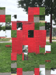
- The image after being scrambled 25 times.
-
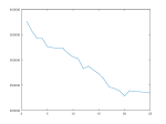
- The consistency score as a function of the number of scrambles.
Having made this observation, I set out to measure what it is that’s changing as we permute the regions in an image. What I’ve come up with is a tractable, and useful measure of local color consistency that also serves as the measure that ultimately allows the reassembly algorithm to function. At a high level, the algorithm swaps regions in the scrambled image, and tests whether the local color consistency score increased or decreased as a result of the swap, and proceeds mechanistically with the goal of maximizing local color consistency. The images above show the average color of each region in the original image, the image after being scrambled 25 times, and a graph showing the total color consistency score as a function of the number of scrambles (i.e., starting with the original image and randomly swapping regions).
Color, Distinction, and Complexity
As noted, at a high level, the reassembly algorithm operates by maximizing the consistency between the colors contained within two regions. This requires us to measure the similarity between sets of colors, which in turn requires that we measure the similarity between individual colors.
Because colors are typically represented as RGB vectors, it’s both natural and convenient to measure the difference between two colors using the norm of the difference between their corresponding color vectors. However, for purposes of the reassembly algorithm, we’ll also have to be able to say whether we should distinguish between two colors. That is, we’ll have to develop a binary test that determines whether or not two colors are similar enough to constitute a “match”.
This question cannot be answered by looking only to the norm of the difference between two color vectors, since the norm operator will produce only a measure of difference. That is, on its own, this difference cannot tell us whether we should distinguish between the two colors. This is essentially the same question that I answered in the development of all of my algorithms, which is, given the context, what is the minimum sufficient difference between two objects that justifies distinguishing between them?
Distinction is what drives complexity, both as a practical, and theoretical matter. That is, the more granular our distinctions are, the more complexity any observed object will have, and the less we distinguish, the less complexity any observed object will have. Though the actual algorithmic complexity (i.e., Kolmogorov Complexity) of an object is not computable, we can get close enough using the Shannon entropy, which is a built-in function in both Matlab and Octave.
As a result, we can find a useful answer to the question of what minimum difference justifies distinguishing between two objects in a dataset by iterating from 

The core observation that underlies nearly all of my work in artificial intelligence is that the value of 
Imagine adjusting the focal point of a camera lens – at all focal points before and after the correct focal point, the image is simply blurry, suggesting that the rate of change in structure is probably roughly the same on either side, until you approach the actual focal point, when suddenly, a drastic change in perceived structure occurs. Though this is not a mathematically precise analogy, it is useful for establishing an intuition for why this approach works as a general matter.
The “Delta-Intersection” of Sets
The algorithm measures the similarity between two regions in an image by counting the intersection of the sets of colors contained in the two regions. Ordinarily, intersection is measured by counting the number of common elements contained in two sets. In this case, we treat two colors as “the same” for purposes of calculating the intersection, so long as the norm of the difference between their respective color vectors is less than
The object whose complexity we’re measuring is in this case a matrix that contains the intersection count between a given region and its four neighbors (up, down, left, and right). That is, each region in the image can be associated with a row and a column index 
Note that as we ratchet up the value of
In calculating the entropy of the matrix, we treat the intersection count in each entry as a frequency, divide by the total intersection count across all entries, and then treat the resulting set of numbers as a probability distribution. This means that as the intersection count becomes more uniform across the image, the entropy of the matrix will increase. In turn, this means that images that are uniformly color-consistent will have a high entropy, whereas images that have pockets of highly consistent regions, and other pockets of less consistent regions, will have lower entropy. This is similar to how entropy is used generally, as a measure of dispersion, but in this case, the quantity whose dispersion we are measuring is the intersection count as a portion of the total intersection count over the entire matrix.


The results of the algorithm of course depend upon the complexity of the image, and as the example above shows, it does produce errors with more complex scenes, and fails to recognize some of the obvious outlier regions. Nonetheless, it clearly uncovers a significant portion of the original structure of the image, and moreover, I expect to be able to improve its performance without significantly impacting runtime by tweaking some of the underlying variables, such as the number of colors it samples in each region.
After I’m convinced that I’ve maximized its performance, I’m going to follow up with a more formal working paper that measures the performance of the algorithm, and possibly, present other applications of this algorithm outside of image reconstruction. But for now, I can say that it is a very low-degree polynomial runtime algorithm (I believe 

I’ll also follow up with a new image partition algorithm that makes use of the
The relevant Matlab / Octave code can be found in the Algorithms tab (see, “unsup_image_rebuild_fast”). Subroutines can be found by typing the function name in the search field on my code bin.
 ; and then extracted the center
  , where
  is the length of the segment, and
  is the velocity of the segment. Because
  is finite.
 and
and  , both of length
  . Because
  . The amount of time it takes for this gap to cross the sensor is
  , which will obviously depend upon the velocity of the segment. If we assume that the light turns off once the sensor hits this gap, then the amount of time the light is off during this gap will vary with the velocity of the segment.
 , in short, it gives us the energy of a single “parcel” of light
  , known as a photon, as a function of its frequency
  . The constant
  is known as Planck’s constant, given that Max Planck penned the equation, though Einstein also had a role in popularizing the view that light is “quantized” into photons through his work on the photoelectric effect.
 . We showed below that we can explain this phenomenon, as well as other related phenomena, by assuming that what is perceived as luminosity is actually a representation of the amount of information observed. That is, the perceived brightness of a light source is not a direct representation of the luminosity of the light, but is instead a representation of the amount of information required to represent the luminosity of the source. In crude (and imprecise) terms, if the luminosity of a light source is 10, then we need
  bits to represent its luminosity, meaning that what we perceive as brightness should actually be measured in bits.
 .
.![W = \sin[\pi (f - f_{min}) / (f_{max}- f_{min})]](https://s0.wp.com/latex.php?latex=W+%3D+%5Csin%5B%5Cpi+%28f+-+f_%7Bmin%7D%29+%2F+%28f_%7Bmax%7D-+f_%7Bmin%7D%29%5D&bg=ffffff&fg=444444&s=0&c=20201002) ,
, is the frequency of the photon in question,
  is the minimum perceptible frequency (i.e., the minimum visible frequency of red) and
  is the maximum perceptible frequency (i.e., the maximum visible frequency of blue/violet). Combining these two equations (but dropping the constant), we have the following equation relating the frequency of a photon to its perceived luminosity:
![L_P = \log(f) \sin[\pi (f - f_{min}) / (f_{max}- f_{min})]](https://s0.wp.com/latex.php?latex=L_P%C2%A0%3D+%5Clog%28f%29+%5Csin%5B%5Cpi+%28f+-+f_%7Bmin%7D%29+%2F+%28f_%7Bmax%7D-+f_%7Bmin%7D%29%5D&bg=ffffff&fg=444444&s=0&c=20201002) .
. THz and
  THz, we obtain the attached graph.
