In a previous research note, I showed how to use my deep learning application Prometheus to do video classifications. The technique I employed was to apply image classification to each frame of the video, which produces a vector of classifications for each video file. That is, a video consists of some number of frames, and so if we classify each frame as an image, we will generate a vector of classifications that contains as many entries as the video contains frames.

I’ve been experimenting with broadening this approach, by repeatedly applying my classification and prediction algorithm. Specifically, I build a first model using the “generate data tree” function, as applied to a portion of the training set. Then, I take a new portion of the training set, and feed it to the prediction algorithm, which will generate classification predictions. However, during this process, it compares each input to every entry in the data tree that underlies the prediction model. By saving saving this information in a vector, we’ll generate a vector of differences associated with each input.

We can then classify those vectors of differences, by calling the “generate data tree function” again, using those vectors as the training dataset. If we do this repeatedly, we’re going to generate a chain of models, and we can then pump new testing inputs through that chain, generating a classification prediction at each stage of the chain. The end result of this process will be a vector of classifications: the same product produced by my video classification technique. We can then classify those vectors of classifications, with the expectation that this final classification will make use of multiple layers of information extracted from the original dataset.

We could also generate a chain of length three, and then put the bottom two models in the chain into a loop. That is, if the models are M1, M2, and M3, we could run the output of M3 back into the input of M2, producing a loop that would run some fixed number of times, generating a fixed number of classifications. This would cut down on model generation time, but still allow us to generate a vector of classifications. You need a minimum of three models to do this because the input to M1 is the actual training data, whereas the inputs to M2 and M3 are vectors of differences.

I’m also going to experiment with random “filters”, rather than using the trees generated during this process. That is, we compare the vectors to randomly generated vectors, measure the differences, and store them as a difference vector. The hope would be that each class will have a signature pattern when applied to the same set of filters.

I’m currently testing this and will follow up in the next few days with code and a research note.

In a previous research note, I introduced a method of delimiting sequences of data, by testing the ratio of adjacent entries in the sequence. This process generates mutually exclusive categories, simply because it places delimiters in the sequence of data, which we can then interpret as indicators that mark the beginning and end of categories. I showed how this method can be used to quickly find the boundaries of objects in images, and of course, it can also be used to categorize data.

However, rather than read the data in the order in which it is presented, we can also compare each element to every other element, thereby generating non-mutually exclusive categories. That is, you perform the same process that I described in the previous research note, but rather than simply test adjacent entries, you test a given entry against all other entries in the dataset, as if they were adjacent. This will generate a category for each element of the dataset. We then test each element, against every other element, and if the test generates a delimiter, then we don’t include the element in question in the category in question. If the test does not generate a delimiter, then we do include the element in question in the category in question.

We can of course also produce mutually exclusive categories using this technique by simply tracking which elements have already been selected.

In the research note below this one, I noted that there is good reason to believe that there is a single objective in-context minimum difference for distinction, which I call , and that two of my categorization algorithms produce very similar values for when applied to the same dataset, despite the fact that the algorithms are very different. Specifically, one produces mutually exclusive categories, and the other produces non-mutually exclusive categories. Nonetheless, both produce very similar values of

The question is then, does the delimiter process, which also produces a measure of distinction I call , produce roughly the same value for , whether we’re generating mutually exclusive categories, or non-mutually exclusive categories?

I’m going to test this hypothesis over the next few days, and follow up with the results.

Since it’s easy to generate either mutually exclusive categories, or non-mutually exclusive categories using this approach, regardless of the operator we use to compare two elements of a dataset, it suggests a more general question:

Is there is an objective, in-context level of distinction associated with every operator as applied to a dataset?

My original categorization algorithm uses the norm of the difference between two vectors to compare elements of a dataset. But my library contains algorithms that use other operators, such as intersection, inequality, and we can imagine others, like taking the union of sets. These are just trivial variations on my main theme of AI, which is to iterate through levels of distinction, and select the level that generates the greatest change in the entropy of the object in question.

Restating the question: is there a single, objective threshold value, analogous to , that is associated with every operator as applied to a given dataset?

To test this hypothesis, we’d have to generate mutually exclusive categories using the operator in question, note the associated value of , and then generate non-mutually exclusive categories, and compare the resultant value of to the prior value of . I will test this hypothesis as well, but possibly in a separate note, since it is a much larger topic.

Even if two datasets are derived from the same pool of observations, it could still be the case that there are unaccounted for differences between the two datasets that are not apparent to a human observer. Any such discrepancies could change the way we think about the data, and could, for example, justify building two separate models, or suggest the existence of inconsistencies in the way the datasets were generated, undermining the validity of any inferences drawn from the datasets. Below, I’ll show how we can use one of my algorithms to measure the internal consistency of a single dataset, and the consistency between two datasets.

Measuring Internal Consistency

In a previous article, I mentioned that I had written an algorithm that can quickly generate non-mutually exclusive categories on a dataset. Like nearly all of my algorithms, this “graph categorization algorithm” generates a measure of distinction , that tells us how different two data points need to be in order to justify distinguishing between them in the context of the dataset. Specifically, if vectors and are both in some dataset, then we distinguish between and only if . That is, if two vectors are within of each other, then we treat them as equivalent, whereas if the norm of their difference exceeds , then we distinguish between them.

The structure of the dataset will of course affect the value of . Generally speaking, if the data is spread out, then will be large, and if the data is concentrated, then will be small. As a result, when we add new data to a dataset, we will almost certainly change the value of . However, if we add new data that is drawn from the same underlying dataset, then the value of shouldn’t change much. That is, if the original dataset is sufficiently large, then we’re not learning anything from the new data – we’re just including more examples of the same type of data. As a result, we can use as a measure of how much the inclusion of new data changes the structure of a dataset, by evaluating before and after the inclusion of the new data.

Let’s begin by incrementally adding new data to a dataset, and measuring the value of at each iteration. The dataset will in this case consist of 10-dimensional vectors of random numbers generated by Octave. The expectation is that the value of should stabilize once the dataset is sufficiently large, since once we have enough data, the appropriate level of distinction should become clear, and roughly invariant with respect to new data being added. Stated differently, assuming my algorithms work, there should be a single level of distinction for a dataset, that shouldn’t change as we add new data, assuming the new data is of the same type as the existing data.

We can accomplish this with the following Octave code:

N = 10;

for i = 1 : 500

data_matrix = rand(i,N);

[final_graph_matrix final_delta] = generate_dataset_graph(data_matrix, N);

data_vector(i) = final_delta;

final_delta

endfor

figure, plot(1:500,data_vector)

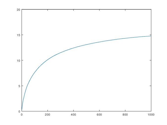
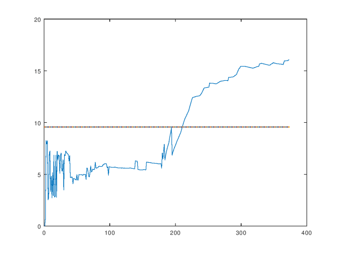
This will add one new vector at a time to the dataset, categorize the dataset using the “graph categorization algorithm”, print the resultant value of , and store it in a vector that is later displayed as a graph. Below is the graph generated by the code above, which will vary somewhat each time you run the code, since the dataset is generated randomly. Note that even though the graph categorization algorithm is fast, and has a polynomial runtime, the code above involves calling the algorithm times, so it’s going to take a little while to run. I’ve named the graph generated by plotting as a function of the size of the dataset the consistency curve for the dataset. The average over the consistency curve is in this case , and the standard deviation is .

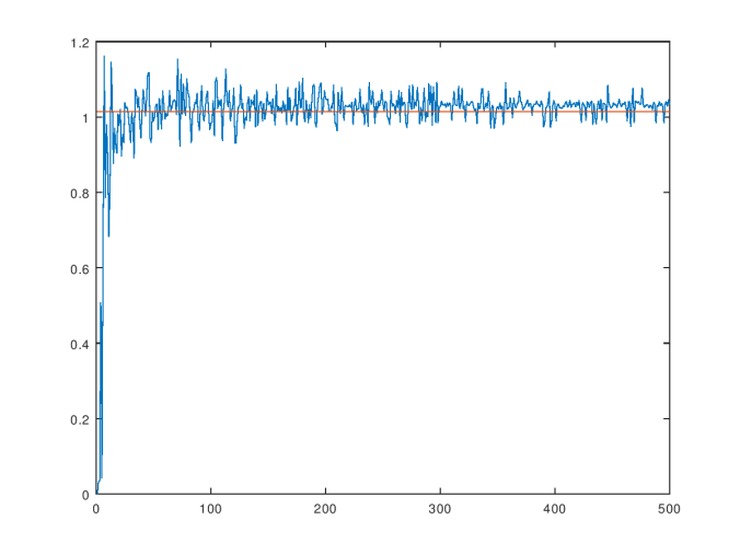
The consistency curve for the dataset of random vectors.

As you can see, the value of stabilizes near the average, which is shown as the orange line in the graph above. This result is consistent with the hypothesis that there should be a single objective value of that is intrinsic to the dataset in the abstract, and not dependent upon the number of observations. Obviously, without a sufficiently large number of observations, you can’t determine this value. But nonetheless, at the risk of being overly philosophical, there really is an underlying process that generates every dataset. Therefore, the correct minimum difference that warrants distinction in the context of a particular dataset is a function of that process, not the observed dataset. The observed dataset gives us a window into that process, and allows us to generate an approximation of the true, underlying in-context difference that warrants distinction between observations generated by that process.

The idea that there is a single, in-context measure of distinction for a dataset is further supported by the observation that replacing the graph categorization algorithm, with my original categorization algorithm (“optimize_categories_N”), in the code above produces very similar values for . This is actually remarkable, because these two algorithms make use of different processes, and generate different outputs: the graph categorization algorithm generates non-mutually exclusive categories, whereas the original categorization algorithm generates mutually exclusive categories. Nonetheless, they generate approximately the same values of , which supports the notion that just like a dataset has a “true” mean, and standard deviation, there is also a true minimum difference that warrants distinction – i.e., a true value of .

It also supports the idea that my method of selecting the level of distinction that generates the greatest change in the entropy of the object in question is the correct way to find this value of , since this is the method that both algorithms have in common, despite the fact that they produce different outputs using that value of .

Now let’s repeat the same process using the Wine Dataset, which is courtesy of the UCI Machine Learning Repository. The same hypothesis should hold, which is that the value of should stabilize around the “correct”, in-context level of distinction for the dataset as we add more data. This is in fact exactly what happens, as you can see in the chart below. The average value over the consistency curve is in this case , and the standard deviation is .

The consistency curve for the Wine Dataset.

The volatility of the consistency curve should decline as a function of the number of observations, and if it doesn’t, then this implies that new observations carry new information about the structure of the dataset. Since this could of course be the case, not all datasets will produce consistency curves that stabilize, and so we can use this curve as a measure of the internal consistency of a dataset. That is, the greater the volatility of this curve, the more “shocks” there are to the structure of the dataset from new observations. If this persists, then there might not be a single process at work generating the data, which means that what we’re observing might actually be transitory in nature, and not a stable process that we can observe and predict. Alternatively, it could be the case that the underlying process has a high complexity. That is, if the underlying process has a high Kolmogorov complexity, then it will generate a large number of novel observations, each of which will shock the dataset. Finally, the dataset could also contain interjections of noise, which will also shock the dataset if the noise is novel every time, which is plausible, since noise is presumably the product of a Kolmogorov-random process that generates novel observations.

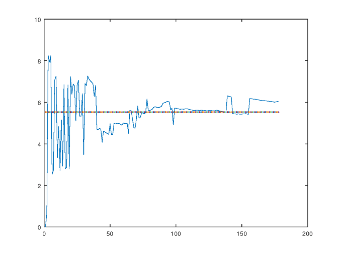
The consistency curve for the Ionosphere Dataset.

Above is the consistency curve for the Ionosphere Dataset, which is also courtesy of the UCI Machine Learning Repository. The average over the curve is , and the standard deviation is . As you can see, it’s highly volatile, suggesting that new observations significantly change the structure of the dataset. Interestingly, this dataset produces a large percentage of “rejected” inputs when my prediction algorithm is applied to it. A rejected input indicates that the prediction algorithm believes that the input is beyond the scope of the training dataset. If a dataset is not internally consistent, then randomly selected observations are more likely to be novel observations, and therefore, outside the scope of the training dataset. Therefore, we would expect a large percentage of rejections for a dataset that is not internally consistent, which is exactly what happens in the case of the Ionosphere Dataset.

It’s tempting to think that a countably infinite number of observations (which is obviously not physically possible), would allow us to discern the “true” level of distinction using this process, but I’m not sure that’s correct. I haven’t worked through the mathematics carefully, yet, but even a superficial analysis implies that the notion of entropy has to change when you have a countable set, since Shannon’s equation does not work with a countable set. Specifically, you can’t have a uniform distribution on a countable set using ordinary probabilities, and therefore, you need a new measure of entropy if you’re going to make use of countable sets. But, as far as we know, observation is finite, so this question is academic, at least for now.

Measuring Consistency Between Datasets

If we have two datasets of observations that were ostensibly generated using the same procedures, and sampled from the same source, then the value of shouldn’t change much when we combine the datasets. If does change significantly, then either the two datasets are incomplete on their own, or, there’s some underlying difference between them that’s unaccounted for.

There are probably a number of reasonable ways to go about testing the consistency  between two datasets using , but the method I’ve decided to use is to generate three consistency curves: one for the first dataset, one for the second dataset, and one for the combined dataset. Then, we can measure both the average value and standard deviation of each consistency curve. When examining the consistency curve for the combined dataset, if it turns out that the average value changes significantly, or the standard deviation increases significantly, in each case as compared to the two individual curves, then it suggests that combining the datasets significantly disturbed the structure of the individual datasets. This in turn suggests that the two datasets are in fact distinct. In contrast, if the average value of is not significantly changed, and the standard deviation is unchanged or decreases, then it suggests that the two datasets are consistent.

If the two datasets are both reasonably large, and their individual consistency curves stabilize, then if the combined consistency curve is drastically more volatile, we can be more confident that the datasets are not incomplete, but that instead, there is some bona fide difference between them. If they’re both sampled from the same source, then there must be some difference in the sampling process that explains the resultant differences between the datasets. As a result, we can also use this process to identify inconsistencies in sampling methods used to gather data, as well as distinguish between datasets that are superficially similar, but nonetheless have some subtle differences that might not be apparent to a human observer.

We’ll apply this process by combining the Parkinsons Dataset, which is again courtesy of the UCI Machine Learning Repository, and the Wine Dataset. The Parkinsons Dataset is dimensions, and the Wine Dataset is dimensions. As a result, we can’t combine them without reducing the dimension of the Parkinsons Dataset to . Reducing the dimension of the Parkinsons Dataset will obviously affect the dataset, but we’re using it for a very limited purpose, which is to demonstrate that when two datasets that are clearly not consistent with each other are combined, the consistency curve will be drastically impacted.

The consistency curve for the Parkinsons Dataset, limited to .

Above is the consistency curve for the Parkinsons Dataset, limited to dimensions of data. The average over the curve is , and the standard deviation is . Though there are some shocks, it trends reasonably close to the average, suggesting that the dataset is reasonably internally consistent, even when limited to dimensions. Below is the consistency curve for the Parkinsons Dataset using the full dimensions of data. The average over the curve below is , and the standard deviation is . The inclusion of the additional dimensions obviously affected the consistency curve significantly, but this was expected.

The consistency curve for the Parkinsons Dataset, using all dimensions.

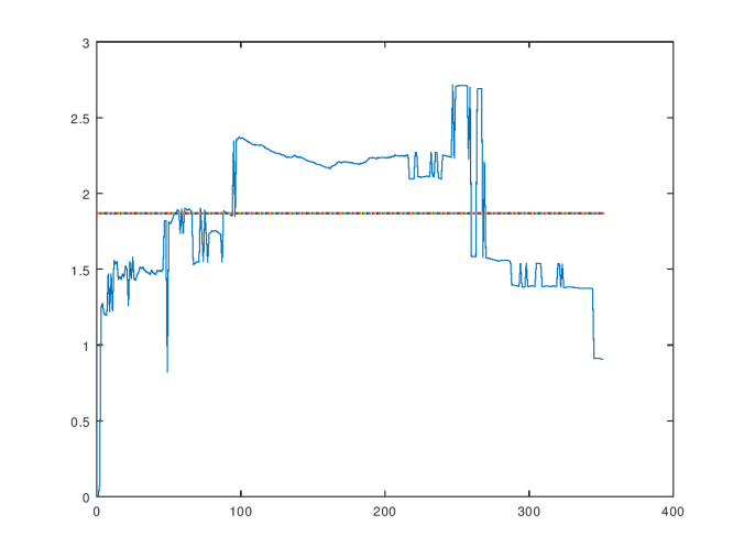
I combined the two datasets into a single dataset with the rows from the Wine Dataset first, and the rows from the Parkinsons Dataset afterward, without changing the order of the rows in either dataset. I then ran the same process on the combined dataset, which generated the consistency curve below. The Wine Dataset contains rows, and the Parkinsons Dataset contains rows, and you can clearly see that the consistency curve breaches the average after roughly observations, suggesting that the inclusion of the Parkinsons Dataset drastically altered the dataset, which is consistent with our hypothesis. The average over the curve is , and the standard deviation is .

The consistency curve for the combined dataset.

Deciding whether two datasets are distinct is a binary question, but the purpose of this process is to provide data that informs a decision either way, rather than an objective threshold for distinction. In this case, the results are rather obvious. Nonetheless, the decision to distinguish will depend upon what you’re doing with the data. That is, even if there’s a significant degree of inconsistency between two datasets, it might not matter for certain purposes, which means that we can’t set an objective point at which distinction is necessary, without also taking into account the purpose for which the datasets are being used.

This process of comparing consistency curves could be a powerful tool for statisticians looking to identify errors and inconsistencies in their sampling procedures, and for data scientists deciding whether to build separate models for ostensibly similar datasets. Though it’s not an area of interest for me, I suspect this methodology could also be used to facilitate forgery detection, and DNA analysis, since this process would uncover discrepancies in superficially similar datasets, which could be generated by examining real-world objects.

Applications to Data Compression

If we have an extremely large dataset, then we probably don’t want to use the entire dataset as a training dataset, since this will require a significant amount of time, and, at least when using my software, generate a large model (i.e., the data structure that models the dataset will be large). A large model will slow down predictions, so for both reasons, we should use as little data as possible in training the learning algorithm.

In order to compress a dataset, we could randomly select data from the dataset until the consistency curve stabilizes. Once the consistency curve stabilizes, we can form the reasonable expectation that there shouldn’t be any further shocks to the sampled dataset from new observations, and therefore, any new information from the dataset will be of only marginal importance. Of course, this could be wrong, and there could be some corner of the dataset that is significant, that we just happened to miss in our sample. But nonetheless, as a practical matter, this should work just fine, and if at some future point our model starts to generate a significant number of errors, then we can retrain it.

Changes in Entropy; Physics

For those that are interested in further reading, in a previous article, I discussed how the entropy of a dataset changes as we add new data. The results are similar to the results presented above, and actually form the basis of my prediction algorithm. For those interested in making sense of the Kolmogorov complexity of a physical process, you can see my paper on the applications of information theory to physics, though it is quite long.

My main categorization algorithm that underlies Prometheus generates mutually exclusive categories. But we can use a similar method to generate categories that aren’t mutually exclusive. Specifically, we can generate a value , and then ask, as a general matter, whether two elements of a dataset are within of each other. Represented visually, we can assign each data point in the dataset a vertex in a discrete graph, and if two data points are within of each other, then we connect them with an edge.

We can generate using my main categorization algorithm, which will produce an in-context value of , or we can instead use another technique I introduced previously that measures the local consistency of data. Using the local consistency technique, if we have elements in our dataset, we would produce an matrix, where entry is only if data points and are within of each other.

We would then iterate through different values of , and select the value that generates the greatest change in the entropy of the matrix. For an explanation of why this would work, you can have a look at my main research paper on AI.

This will produce a category associated with each element of the dataset, where another element is a member of that category only if it is within of the element that defines the category.

We can use the resultant matrix to define a graph that is associated with the dataset. This graph will show, visually, which data points are sufficiently similar to be connected by an edge, which in turn allows for the quantization of distance by path length between all elements of the dataset.

The script to generate this categorization / graph is available on my researchgate blog.

There are other variations on this theme that we could use, like calculating a measure of the entropy of the graph, rather than the entropy of the matrix that defines the graph, but this works, and so, that’s it for now.

I plan to use this technique in a real-time deep learning algorithm called Ayin ( ע ) that I’m currently working on, which should (hopefully) be ready in the next few days. I will also further optimize my existing algorithms to make maximum use of vectorization, which I hope will push performance over the edge, allowing for truly real-time deep learning on consumer devices.

I’m happy to announce that a free, non-commercial version of my Prometheus Deep Learning Engine is now available as a GUI Application.

Below / Attached is a research note that explains how to use Prometheus to do basic machine learning, and deep learning video classification.

Everything you need to download, and install Prometheus, can be found in the research note:

https://www.researchgate.net/publication/335224609_Autonomous_Deep_Learning

If you’re interested in purchasing a commercial version of Prometheus, please send me an email using the email address on my SSRN page.

Autonomous Deep Learning

I’ve put together a command line interface that allows for autonomous machine learning and deep learning using my AI algorithms:

https://www.researchgate.net/project/Information-Theory-SEE-PROJECT-LOG

The user simply selects the training file and testing file using a GUI, and a single core learning algorithm automatically generates a model, and then predictions. I’ll follow up with a research paper demonstrating how this one application can do everything from basic machine learning, to deep learning video classification.

I’m also working on a full blown industrial quality Python application, that will allow for GUI-based access to all of my AI algorithms, ultimately allowing non-experts to do the work of machine learning and deep learning, simply because it’s so easy to do using my algorithms. With the addition of a GUI, only minimal training will be necessary to accomplish otherwise very sophisticated tasks in AI.

The business case for this application is obvious: you don’t need as many data scientists when you have an application that can spontaneously generate models that work fast and accurately. Shrewdness aside, this will also allow data scientists to leverage the power of this application to do things that were simply impossible beforehand, and focus on more interesting questions.

If you’re interested, or know someone who would be interested, please send me an email. You can find my email address by clicking the “Contact” button on my SSRN page.

Note that if you’re using my algorithms on a dataset where the dimensions contain drastically different values, then performance could be negatively affected. One simple way to identify this problem, is to measure the standard deviation of the log base 10 of each dimension of the dataset.

So for example, if a row contains the entries [1 10 100], we would calculate log([1 10 100]) = [0 1 2], and then calculate the standard deviation of that vector, which is in this case 1. If the standard deviation of this vector is above 1, then you should probably experiment with weighting the data before training the algorithms. This can be done by a simple loop that divides the outlier large dimensions by powers of 10, and then tests the resultant accuracy, of course picking the weights that generate the greatest accuracy.

On a related note, I’m generalizing my statespace optimization algorithm to allow for totally arbitrary input data, where the algorithm will decide on its on how much to weight a particular dimension of a dataset.

Note that this is not what gradient descent and other interpolation algorithms do. Those types of algorithms use the weights to classify or predict data. My AI algorithms can already simulate basically any machine learning or deep learning algorithm as they stand.

This additional step will instead allow my algorithms to identify which dimensions are relevant when given a dataset that might contain a significant amount of irrelevant information (i.e., a significant number of “noise” dimensions), as opposed to unbalanced but relevant “signal” dimensions. That is, this process will allow my algorithms to autonomously identify which dimensions from a dataset are most relevant, and then construct categories using those dimensions.

Shannon’s entropy equation can be used to solve resource management problems:

Let’s say we have 5 nodes in a search space, and we expect each node to be about the same distance from some goal state. In this case, there’s no reason to allocate more computational resources to one node than any other, since ex ante we expect all nodes to perform the same.

Now imagine that we expect one of those nodes to be significantly closer to the goal state than the others. It would be rational in that case to dedicate more computational power to the states generated by that node.

We can use Shannon’s equation to answer the question of how much additional power should be allocated.

We can also use information theory to help guide the search process itself. If we know nothing about a state-space, we’ll probably want to fully unpack all the nodes until we have a robust set of nodes that have some minimum threshold of diversity.

Generating that last, sufficiently diverse state-space will of course necessarily require producing a sequence of state-spaces, each with their own measure of entropy.

We can then apply my standard technique in AI, which is to select the state-space that generates the greatest change in the entropy of the state-space during that process.

This is the state-space that produced the greatest change in the structure of the state-space, which we can then use as our starting point for more carefully unpacking the depths below.

Finally, generating a state-space is generally very computationally intensive, and likely to be exponential as a function of the number of iterations (i.e., a state-space can be represented as a tree with an exponentially wider breadth as a function of depth). As a result, it’s rational to try and compress the number of dimensions used in navigating the state-space.

I introduced an approach to dimension compression in the note below this one that makes use of my categorization algorithm, but one possibly faster approach is to simply test how sensitive the value we’re attempting to predict is to changes in the input dimension in question. That is, we would start with dimension 1, and test the response of the function we’re evaluating to changes in the value of that dimension, and repeat this process for each dimension. Then, we allocate resources according to how sensitive the output variable is to the dimension in question.

So for example, if we’re trying to find the minimum of the function , the value of is going to be far more sensitive to changes in the value of than changes in the value of . This is easy to test, so we can do this type of test quickly for each dimension of a dataset, and then allocate resources using Shannon’s equation (where the most sensitive dimensions get the most resources), or simply select some fixed number of the most sensitive dimensions. This could dramatically reduce the workload of the state-space navigation function for high-dimensional functions.

 I’ll follow up with code and a research note.

In a previous research note, I introduced a method of quickly calculating an expectation value for the intersection count between any two given sets randomly selected from a family of sets. I’ve been doing work on the MovieLens dataset, and though I’ll soon post a more fulsome research note on the matter, I realized that the expected intersection calculation can be used to measure how much mutual information is contained on average between vectors in a dataset.

For example, the MovieLens dataset consists of around 200,000 movies rated by 610 users. However, a given user generally rates only a small fraction of those movies. We could simply take the entire dataset, but because it’s 200,000 dimensions, this will impact performance, and because each user doesn’t generally rate all of the movies, we’re probably doing far more work than is necessary. That is, we can almost certainly find a subset of those 200,000 dimensions that will give us enough information to meaningfully analyze the dataset.

The solution I’ve come up with is to sort the movies in the order of how many ratings they receive. That is, the top of this list is the movie that was rated by the most users. This is not necessarily the most popular movie, but rather, the movie that the most users took the time to rate.

As we proceed down this list, the probability that a given user rated the movie in question declines. As a result, each movie contributes less and less to the information about the dataset as we move down the list, simply because, by definition, fewer users have reviewed it.

We can then, for example, take a subset of the original dataset that corresponds to the top 100 movies in terms of their review count. Again, these are not necessarily the 100 most popular movies, but are instead the top 100 movies in terms of how many people reviewed them.

Even though these are the most rated movies, it’s still possible that the resultant subset of the dataset contains missing data. That is, just because a movie is frequently rated, doesn’t mean that all users rated it.

If we shape the dataset as a data matrix where each row corresponds to a user, and each column in a given row contains the rating the user gave to a particular movie, then we can then test which column entries are non-zero (i.e., non-empty), which will produce a binary matrix, which we can then feed to the expected intersection algorithm. This will calculate the expected number of overlapping, non-empty entries between any two rows from the dataset.

This is, therefore, a measure of the number of overlapping dimensions we’re expected to have between any two vectors from the dataset (i.e., any two rows from the data matrix).

We can then iterate the number of top movies sampled, and then measure the expected intersection count for each resultant subset of the dataset, which will allow us to measure how much information we’re getting in return for adding dimensions to our dataset. Below is a chart showing the expected intersection count for the MovieLens dataset as a function of the number of dimensions, where dimensions were added in the order of their rating count (i.e., dimension one is the most rated movie).

Dimension Compression

There is, however, no objective stopping point to this process. That is, the expected intersection between dimensions will continue to increase as we add more dimensions, and though we can measure the derivative of this function, there’s no obvious point at which we can say, this is the “right” amount of overlap between dimensions.

We can, however, apply my categorization algorithm (or some other categorization, or clustering technique) at each iteration, measure the entropy of the categorization, and find the number of dimensions that generates the greatest change in the structure of the categorization.

This is exactly what my core categorization algorithm does, except in that case, entropy is measured as a function of the level of distinction, . In this case, we’d be measuring the rate of change in the entropy of the categorization as a function of the number of dimensions used to generate the categorization.

So in short, we sort the dimensions of a dataset by frequency as described above (i.e., the most commonly used dimensions go first), and begin by categorizing the data using only the most common dimension (or some other small number of dimensions), and measure the entropy of that categorization. Then, we add the next dimension, categorize the dataset using those dimensions, and measure the entropy of the resultant categorization. We repeat this process up to a predefined maximum, which will presumably depend upon performance constraints. So if the machine in question can handle the full dimension of the dataset, then we can probably iterate up to that full number of dimensions.

Note that at each iteration, we let the categorization algorithm (or other clustering technique) run to fruition, producing a complete categorization of the dataset using the number of dimensions in question.

By selecting the number of dimensions that generates the greatest change in the entropy of the categorization structure, we will select the number of dimensions that unlocked the greatest amount of structure in the dataset – i.e., the most relevant dimensions of the dataset.

Now, it would be fair to say that this process actually requires more work than simply categorizing the data once, using all of the dimensions in the dataset, and that is correct. That is, by definition, this process will repeatedly categorize the dataset for every dimension from 1 up to and including N (i.e., the actual number of dimensions). This is obviously more work than simply categorizing the dataset once using all N dimensions.

However, we can use the expected intersection to select a representative subset of the dataset, and apply this process to that subset, rather than the entire dataset. Specifically, we can randomly select vectors from the dataset, and test the expected intersection for that subset of vectors, and iteratively increase the number of vectors selected until we hit an expected intersection count that is sufficiently close to the expected intersection count for the entire dataset (and sufficiently stable as we add more vectors). That is, we add vectors until the expected intersection for the subset is close to, and stable around, the expected intersection for the entire dataset.

We can also test the individual frequencies of the dimensions from this subset of vectors during this process, which is also produced by the expected intersection function. Specifically, we can calculate the norm of the difference between the frequencies of the subset and the frequencies of the entire dataset.

This ensures that we have a number of vectors with dimensions that overlap approximately as much as the entire dataset (as measured by the expected intersection count), and dimensions with approximately the same frequencies of usage as the original dataset (as measured by the frequencies of the dimensions calculated by the expected intersection function in the “weight vector”).

Put together, this will allow us to find the optimum dimension for the dataset without having to repeatedly categorize the entire dataset. Finally, note that we could apply this process to any resultant data structure capable of generating a measure of entropy. For example, we could apply this process to my  “generate data tree algorithm“, which generates a tree of subcategories of a dataset, measuring the entropy of the resultant data tree after each iteration over the dimensions.

Measuring Missing Information

We can also use these ideas to get a sense of how complete a dataset is by measuring the expected intersection on the full dataset, and dividing by the number of dimensions in the full dataset. For example, if the dimension of our dataset is 100, and the expected intersection over the full dataset (as described above) is 10, then the measure would in this case be .1, or 10%. This means that, on average, only 10% of the dimensions of the dataset will be relevant when comparing two vectors from the dataset, since only 10% of them are expected to overlap.

In the extreme case when the expected intersection is 0, then in some sense, we don’t really have a dataset – we have collection of independent observations. For example, if our dataset consists of two vectors (1,2,{}) and ({}, {}, 1), where {} indicates a missing entry, then there is no overlap between the dimensions of those two vectors. This means that without any other information about what the vectors represent, we can’t compare them. In contrast, if the two vectors were (1,2,3) and (4,5,1), then we can of course compare every dimension of the vectors.

Since the expected intersection allows us to form an expectation value as to the number of overlapping dimensions between any two vectors in a dataset, we can in turn measure the completeness of the dataset.

In the language of the theory of AI that I’ve been developing, I would say that this method allows us to measure the extent to which a dataset provides its own context. When the ratio of the expected intersection and the dimension of the dataset is 1, then the dataset provides the maximum context possible without any exogenous information about the dataset. When the expected intersection is zero, then the dataset provides no context, and is instead, ex ante, assuming no other prior information, a collection of unrelated observations.