Identifying Macroscopic Objects in Massive Datasets

Introduction

Following up on yesterday’s article, in which I introduced an efficient method for clustering points in massive datasets, below is an algorithm that can actually identify macroscopic objects in massive datasets, with perfect precision. That is, it can cluster points into objects such that the clusters correspond perfectly to the actual objects in the scene, with no classification errors, and exactly the correct number of objects.

The goal of this work is to build up to an object identification and tracking algorithm, that can operate with an enormous number of observations, as an analog of my earlier object tracking algorithm, but extended to massive datasets, making use of my latest work.

The first step is to cluster the data using the algorithm I introduced yesterday, which will produce not only an initial set of clusters, but also a value called “delta”, that is the in-context minimum difference necessary to justify distinguishing between to two vectors. There’s a lot of thinking behind this, and it is part of the core of my work in information theory, but the big picture idea is, if we have two vectors x and y, that are part of some dataset A, my algorithms will generate a value associated with A, \delta_A, such that if ||x - y|| > \delta, then x and y are distinct vectors, in the context of the dataset A.

If you’re interested, you can read a full explanation of the theory and mathematics of this process in my original article on A.I., “A New Model of Artificial Intelligence“.

Another property of the value delta, is that it quantizes distance in a dataset. That is, we can express the distance between two vectors as an integer multiple of delta, using the ceiling or floor operator. Now you could of course say, “so what”, since you can do that with any number, but the difference is, delta tells you how far apart things need to be in order to say they’re different in a particular context, which makes it a natural unit of measure for the dataset that generated the value of delta.

The algorithm below makes use of this insight, by doing the following:

First, we generate a value of delta by simply clustering the dataset using the method I introduced yesterday, which will produce additional local clustering. That is, the clusters are accurate, in that points clustered together are actually part of the same object, but the object is overly subdivided. Since the goal is to do object tracking, this is not ideal, and we’d like instead to have clean, macroscopic objects clustered together, that we can then track over some number of frames.

In order to accomplish this, as a second step, we begin with the first vector in the first cluster, which is the minimal element of that cluster. Then, we count the number of vectors that are within 1 \times \delta of this first, minimal element. After that, we count the number of vectors that are within 2 \times \delta, 3 \times \delta, and so on, up to a number of iterations that is calculated in the code, and likely to be modest in number.

If the dataset is comprised of actual objects, then as you get further away from the minimal element of the object, the number of new points should drop off suddenly at the boundary of the object –

Just imagine beginning in the center of a sphere, and proceeding outwards towards the perimeter, counting the number of points along the way. As you do this, the number of new points will increase at a reasonably steady rate, until you reach the perimeter, where the number of new points will drop off to basically zero.

This algorithm tracks the rate of change in new points as you increment the integer multiple of delta, and then finds the point at which the rate of increase drops off, and that’s the boundary of the object.

This is then repeated until the dataset is exhausted.

This could of course work using some other measure of distance, rather than delta, but the utility of this approach is that delta can be calculated quickly for any dataset, so unless you have a different number that you can quickly produce, that works for this purpose, you can’t use this algorithm, despite the fact that it will obviously work.

Application to Data

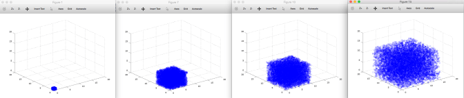
In this case, the dataset consists of 39,314 Euclidean 3-vectors, containing 5 statistical spheres.

Screen Shot 2020-08-05 at 12.37.02 PM

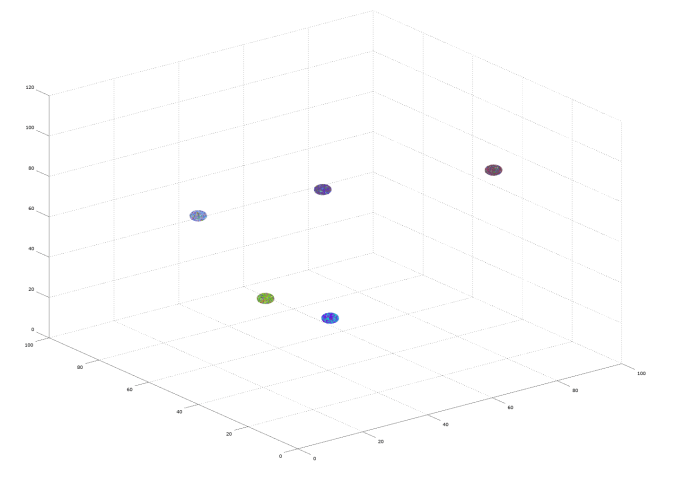
A dataset of five statistical spheres after being clustered.

The initial clustering took 37.2266 seconds, running on an iMac, with no errors, in that if two points are clustered together, then they are part of the same sphere.

However, as noted above, this process produces additional local clustering that we’d like to eliminate, since the goal is to identify and track macroscopic objects. You can visualize this using the image above, in which points colored the same are part of the same cluster, plainly showing multiple colors within the same sphere. The number of clusters produced in this first process is 1,660, suggesting significant local clustering, since there are only 5 spheres.

Screen Shot 2020-08-05 at 12.41.45 PM

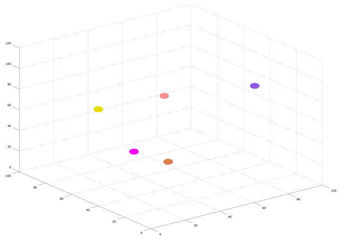
The dataset of five spheres after being subject to macro-clustering.

The next step is to use the value of delta generated in the first step, to try and consolidate these clusters into macroscopic objects.

This next round of clustering took 0.0396061 seconds, running on an iMac, again with perfect accuracy. Moreover, the number of clusters produced is 5, exactly the number of spheres in the dataset, implying that the performance is perfect.

Octave Code:

generate_sphere

vectorized_EMC_clustering_N

EMC_anchor_clustering

Macro_Clustering_CMNDLINE

Full Library:

ResearchGate


Clustering Objects in Massive Datasets

In a previous article, I introduced an algorithm that can quickly find the perimeter of a statistical object that consists of several hundred thousand observations. The goal of this work is to build up to an object identification and tracking algorithm that can operate with an enormous number of observations, as an analog of my earlier object tracking algorithm, but extended to massive datasets, making use of my latest algorithms.

Eventually, I plan to make use of natural language object identification and tracking. For example, the algorithm I’m working on will scan the first scene in a sequence and say, “this is a sphere of radius r”, and then track the scenes going forward accordingly, using the kind of analysis a human being would. That is, rather than cluster points, once all of the objects have been described using human labels in the first scene, those objects will then be searched for in each following scene, using those same human labels, by, for example, looking for a sphere with radius r in each scene, and if there’s more than one such sphere, taking the one that is closest to the original as the next instance of that sphere in the next scene.

The actual identification process will be done using the extremal points of the shape, which can be identified quickly using the algorithm I introduced in my previous article, and then building up a dataset of objects, and the properties of their extremal points. This avoids having to rotate objects for purposes of comparison, and instead, tests for statistical properties that define the shape. For example, the extremal set of a sphere consists of a set of points that are all roughly equidistant from the origin – i.e., the surface of the sphere. You don’t need to rotate the extremal set to figure this out, and as a result, this process should increase efficiency.

I’m probably about a week away from fully developing this algorithm, but as a next step in that process, below is code that clusters objects in a scene, given an enormous number of points in Euclidean 3-space.

Specifically, in this case, the dataset consists of 78,215 Euclidean 3-vectors, that together produce 15 statistical spheres. The classification task is to then cluster the data, so that points within each sphere are clustered together, without any overlap between spheres. This took about 5.4500 minutes, running on an iMac, and you can visualize the resultant clustering below, where points in the same cluster have the same color.

Screen Shot 2020-08-04 at 1.59.35 PM

The data colored by cluster.

There is some sub-clustering within each sphere, which is a consequence of the algorithm, which generates a large number of small clusters, because the data is sorted beforehand for efficiency. However, the actual number of classification errors is exactly zero, in that if two points are clustered together, then they are part of the same sphere.

The next step is to produce follow up code that then clusters the anchors for each cluster, which should produce clusters based upon actual macroscopic objects, rather than the underlying point data, which as you can see, produces some additional local clustering.

Octave Scripts:

vectorized_EMC_clustering_N

generate_sphere

8_4CMNDLINE

Full Library:

ResearchGate

Finding the Perimeter of an Object

In a previous article, I introduced a clustering algorithm capable of quickly handling hundreds of thousands of vectors, that first compresses the vectors to a single dimension using the norm operator.

Though originally intended to cluster velocity scalars, I’ve also used this algorithm to find the perimeter of a statistical sphere, that isn’t smooth or completely solid, which is what you’ll likely end up with using real-world sensor data. In this case, the sphere consists of 327,627 Euclidean 3-vectors. Clustering the data took 4.6819 minutes, running on an iMac, which is all that’s necessary to identify the perimeter of the sphere, since you can then simply select the last cluster in the list of clusters, and color those points in the display. In the image below, the maximum cluster is colored blue, the rest colored gray.

Sphere_Plot

A statistical sphere, with the perimeter colored blue.

Octave Code:

8_2_CMNDLINE

Full Library:

ResearchGate

Nearest-Neighbor on Massive Datasets

In a previous article, I introduced an algorithm that can cluster a few hundred thousand N-dimensional vectors in about a minute or two, depending upon the dataset, by first compressing the data down to a single dimension. The impetus for that algorithm was thermodynamics, specifically, clustering data expanding about a point, e.g., a gas expanding in a volume. That algorithm doesn’t work for all datasets, but it is useful in thermodynamics, and probably object tracking as well, since it lets you easily identify the perimeter of a set of points.

Below is a full-blown clustering algorithm that can nonetheless handle enormous datasets efficiently. Specifically, attached is a simple classification example consisting of two classes of 10,000, 10-dimensional vectors each, for a total of 20,000 vectors.

The classification task takes about 14 seconds, running on an iMac, with 100% accuracy.

I’ve also tested it on two UCI datasets (the “Wine” and “Iris” datasets), and the accuracy was comparable, around 100%, with equally impressive efficiency.

In addition to clustering the data, a compressed representation of the dataset is generated by the classification algorithm, that in turn allows for the utilization of the nearest-neighbor method, which is an incredibly efficient method for prediction, that is in many real world cases, mathematically impossible to beat, in terms of accuracy.

Said otherwise, even though nearest-neighbor is extremely efficient, with a dataset of this size, it could easily start to get slow, since you are still comparing an input vector to the entire dataset. As a result, this method of clustering allows you to utilize nearest-neighbor on enormous datasets, simply because the classification process generates a compressed representation of the entire dataset.

In the specific case attached below, the dataset consists of 20,000 vectors, and the compressed dataset fed to the nearest-neighbor algorithm consists of just 4 vectors.

Predictions occurred at a rate of about 8,000 predictions per second, with absolutely no errors at all, over all 20,000 vectors.

Octave Code:

8-1CMNDLINE

vectorized_EMC_clustering_N

Note that you’ll need to download my full archive to run this code, which you can find on ResearchGate.

N-Dimensional Mass-Clustering

As noted in previous articles, I’ve turned my attention to applying A.I. to thermodynamics, which requires the analysis of enormous datasets of Euclidean vectors. Though arguably not necessary, I generalized a clustering algorithm I’ve been working on to N-dimensions, and it is preposterously efficient:

The attached example takes a dataset of 150,000, 10-dimensional vectors, and clusters them in about 54.2 seconds, with absolutely no errors.

The example is a simple two class dataset, but nonetheless, the efficiency is simply remarkable, and completely eclipses anything I’ve ever heard of, even my own work.

This is particularly useful in thermodynamics, since it lets you cluster points as a function of their distance from an origin, say the center of mass, or the center of some volume. As a result, it allows you to quickly identify the perimeter of a set of points –

Simply take the cluster furthest from the center, which will be last in the list.

So this algorithm is also likely to have applications in object tracking, since you can compress the object to the points at its perimeter, and then track only those points.

This is years into my work, and rather than reexplain things, if you’re interested in how this process works, I’d suggest reading my original paper on machine learning and information theory.

This is another instance of the same ideas in information theory, but in this case, making use of radical compression.

Command Line:

8_1CMNDLINE

Function Code:

vectorized_clustering_EMC_N

Full library:

ResearchGate

Splitting a Dataset

I’m working on the applications of A.I. to thermodynamics, and I had to solve for how to split a dataset into two parts, using objective criteria. Specifically, I’m interested in what’s moving, and what’s not, but the algorithm I came up with is general, and can be used to split any dataset in two, using objective criteria.

It is only a slight tweak on my original clustering algorithm, that requires an additional outer loop that iterates through levels of granularity, because you end up with a coin toss distribution, which produces very slight changes in entropy.

The “final_delta” variable is the threshold value that divides the dataset, so you can test for everything under or over that value, and that’s the dividing line.

The attached code splits a dataset of 50 million real number values in about thirty seconds, running on an iMac.

Command line code:

Split the data

Full set of algorithms:

ResearchGate

Analyzing Microstate Point Data in Thermodynamics

In previous articles, I introduced my algorithms for analyzing mass-scale datasets, in particular, clustering, and other algorithms. However, those algorithms deliberately avoided operations on the underlying microstate data, since these datasets are comprised of tens of millions of Euclidean vectors.

I’ve now turned my attention to analyzing changes in thermodynamics states, which would benefit from direct measurements of the underlying point data in the microstates themselves. At the same time, any sensible observation of a thermodynamic system is going to consist of at least tens of thousands, and possibly millions of observations. My algorithms can already handle this, but they avoid the underlying point data, and instead use compression as a workaround.

In contrast, the algorithm below actually clusters an enormous number of real value points, with radical efficiency, with the intent being to capture changes in position in individual points in thermodynamic systems.

This is a simple example attached that clusters 225,000 real number values in about 120 seconds, running on an iMac –

This is simply ridiculous.

I’m still refining this algorithm, but thought I would share it now, in the interest of owning claim to it.

The accuracy is just under 100%, though this is a simple example.

You could do this a few times on different dimensions independently, and then take the clusters that each dimension produces in common, using an intersection operator, which is extremely fast in MATLAB.

This will allow you to cluster higher dimensional vectors of numbers, though some vectors might end up not getting clustered using this approach. But with this much data, it probably doesn’t matter.

This would in turn allow you to build a prediction model using any of my prediction algorithms. For my model of prediction, you only need one vector per cluster, and in my admittedly limited experimentation thus far, the number of clusters is quite low, implying that prediction should be fast, despite these enormous datasets.

vectorized_EMC_clustering

CMNDLINE 7-28

Using Graphs to Represent Thermodynamic Systems

Attached is software that can generate a graph that represents the transitions of a thermodynamic system, from one state to the next. States that are sequential in time are by definition adjacent, and it’s a directed edge, from the initial state to the next state.

For a thermodynamic system, the underlying state graph is likely to be noise, and mostly disconnected, because microstates could of course occur only once, meaning they have only one next state neighbor.

So in addition, there is code that first clusters the data, into similar states, and then produces a graph based upon items in one cluster transitioning to items in other clusters.

As an example, the attached code uses the expanding gas dataset, over 50 sequences of expansion. So you’d expect the clustering to cause all of the initial states to be clustered together, the later states clustered together, etc, and this is exactly what happens, just as it did in the previous article. As a result, the graph produced should be a path connecting the initial cluster to the final cluster, and this is exactly what happens.

I’ll write some code that allows for visualization of the graphs, but for now, you can examine the matrix to get a sense of its structure:

Screen Shot 2020-07-28 at 11.23.01 AM

The graph matrix for the cluster graph

The integer entries indicate how many items the cluster represented by the row is adjacent to. So entry (1,2) shows that cluster 1 is connected to all 50 states in cluster 2, which is exactly what you’d expect, suggesting that the expanding gas always forms a sequence from one state of expansion to the next.

I’ll follow up later this week, possibly today, with software that then uses these graphs to measure how ordered a thermodynamic system is using graph theoretic measures, such as number of maximal paths, how ordered maximal paths are, etc.

NOTE: I corrected a minor bug in a subroutine related to the dictionary insert function, which is updated and attached.

find_dictionary_index

7_28_CMNDLINE

Measuring Order in Thermodynamics Using A.I.

Clustering Mass-Scale Datasets

In previous articles, I’ve introduced algorithms that can quickly process datasets that consist of tens of millions of vectors, on a consumer device, allowing for meaningful analysis of the microstates of a thermodynamic system.

In the original article on the topic, I showed how my deep learning algorithms can be used to identify the macrostates of a thermodynamic system, given its microstates.

In a follow up article, I showed how to radically compress a dataset consisting tens of millions of vectors into a dataset of just a few thousand vectors, ultimately using this technique to make radically efficient predictions (about 500 predictions per second, running on an iMac), with perfect accuracy, classifying the rate of expansion of a gas.

In this article, I’ll present a method for measuring how ordered a thermodynamic system is, using a combination of techniques from deep learning and information theory. Specifically, I’ll demonstrate how these techniques can correctly identify the fact that an expanding gas has a progression of states, thereby generating an actual, measurable mathematical order as the gas expands, whereas a stationary gas is essentially unordered, in that any microstate of the gas could in theory appear at any point in time.

Order, Entropy, and Variance

Imagine repeatedly watching the same gas expand, from roughly the same initial volume, to roughly the same final volume, with the number of particles being fixed over each instance of expansion. Further, assume that you took some fixed number of snapshots of the system as it progressed from compressed to expanded, at roughly the same relative moments in time.

Now assume you ran a clustering algorithm on the individual states, as observed. Intuitively, you would expect all of the final, most expanded states to get clustered together, since they are the most similar, structurally. Similarly, you would expect all the initial, compressed states to get clustered together, again, because they are the most similar, structurally.

Now, instead of using typical classifiers, let’s instead put the index at which the state occurs in a hidden dimension. So for example, the first state of an instance of the gas expanding will have a classifier of 1, the second state 2, etc. Since each state of the gas will have a classifier that tells us when it occurred, this will create a distribution of timestamps for each cluster, and if the sequence of observations is truly ordered in terms of timing, then all of the states clustered together should occur at exactly the same timestamp (assuming a relative time stamp, expressed as a length of time since the inception).

So for example, in a truly ordered system, all of the initial states would be clustered together, with no other states; all of the secondary states would be clustered together, with no other states, etc. This is probably not going to work perfectly in the case of a thermodynamic system, since the motions of the particles are highly randomized, but nonetheless, intuitively, you’d expect a stationary gas to be less ordered than an expanding gas, since a stationary gas doesn’t have any noticeable macroscopic change, whereas an expanding gas does, since the volume occupied by the gas is increasing.

We can, therefore, use entropy to measure the consistency of the timestamps within a cluster, since the timestamps will literally generate a distribution. For example, assume that an ideally expanding gas is such that all of its initial states get clustered together, with no other states. The timestamps associated with this cluster would look something like \{1, 1, 1, 1, ... ,1\}, if we use simple integer timestamps. This distribution will have an entropy of zero, which indicates perfect consistency. In contrast, if a cluster is comprised of similar states that nonetheless occur at totally different points in the sequence, then the entropy will be non-zero.

For these same reasons, we can also use the standard deviation to measure the consistency of the timestamps associated with a cluster. Returning to the example of the ideal gas, the distribution of timestamps \{1, 1, 1, 1, ... ,1\} will have a standard deviation of zero, whereas a cluster with a diverse set of timestamps will obviously have a non-zero standard deviation.

Together, these two measures allow us to quantify the extent to which a system is ordered, from two different perspectives:

(1) The entropy allows us to measure the multiplicity of outcomes possible;

(2) The standard deviation allows us to measure the variance of when those outcomes occur in time.

Application to Examples in Thermodynamics

As a demonstration, I’ve put together some code attached below that applies these ideas to two datasets:

(A) one is a stationary gas in a fixed volume, represented by 75,000,000 Euclidean three-vectors;

and,

(B) the other is a gas in an expanding volume, also represented by 75,000,000 three-vectors.

The thesis above would imply that the expanding gas is more ordered than the stationary gas, and this is in fact the case.

Beginning with the stationary gas, the first step is to cluster the dataset, using specialized algorithms that I’ve developed to handle enormous datasets of this type –

This takes about 15 minutes, running on an iMac.

Again, rather than attempt to classify the data, we are instead testing for how consistent its positions are in time, so the classifier dimensions are instead integer indexes that tell us at what point in the sequence the state occurred. You could argue that the integers are arbitrary, but this is actually incorrect, and you can use an argument that is similar to the one I use in this article, on the connections between information and error, to show that so long as your observations are always evenly spaced in time, the actual distance in time between observations does not matter for this purpose.

Returning to the measurements described above, we would expect both the entropy and the standard deviation of the expanding gas to be lower than those associated with the stationary gas, and this is in fact the case.

Running the code attached below produced the following measurements:

Stationary Gas:

Average entropy per cluster: 3.9069.

Average standard deviation per cluster: 4.3234.

Expanding Gas:

Average entropy per cluster: 0.87500.

Average standard deviation per cluster: 0.43970.

The command line code is below, and the full archive of my A.I. code is available on ResearchGate.

STAT GAS CMNDLINE

EXP GAS CMNDLINE

Note that you will need to download my archive (approximately 73 MB) to run the command line code.

Predictions Using Mass-Scale Data

Following up on the previous article below, attached is an updated command line script that allows for efficient predictions over datasets comprised of tens of millions of observations in Euclidean space.

The specific dataset in the command line code attached models a gas expanding in Euclidean space, at two different rates of expansion, and the prediction task will be to correctly identify the rate of expansion, as either the, “fast one” or the, “slow one”.

Each state of the gas is comprised of 10,000 points in Euclidean space, and each sequence of the gas expanding consists of 15 states, for a total of 150,000 three-dimensional vectors per sequence.

Screen_Shot_7_22

Four frames from one sequence of the gas expanding.

There are 300 sequences, for a total of 45,000,000 three-dimensional vectors.

Obviously, it is, as a general matter, very difficult to analyze datasets that involve this many vectors, but the algorithms I’ve developed can nonetheless quickly and efficiently cluster and then make predictions over datasets of this type, on an ordinary consumer device.

The first step is to sort the data using an operator I introduced in this article, specially designed for mass-scale data –

This first step took about 10 minutes, running on an iMac.

The next step, is to embed each state of the gas on the real number line, using algorithms I introduced in this article

This step will drastically compress the dataset, from 45,000,000, three-dimensional vectors, to 300, 15-dimensional vectors, with each vector representing a sequence of states of the gas expanding, which took about 25 seconds.

The next step, is to cluster the real-number vectors, which took about .06 seconds.

The final step, is to actually make predictions, which in this case took a total .70 seconds, over the entire dataset of 300 sequences.

The accuracy is in this case perfect with absolutely no errors, given only the first 5 of the 15 observations in each input vector. That is, if you give the prediction algorithm the first 5 states of the gas, it can correctly classify its expansion rate, every time.

My complete set of algorithms is available on ResearchGate, though I’ve also attached the command line code for this particular dataset as a PDF.

7-22CMNDLINE