You and I (Music)

April 13, 2021 / erdosfan / Leave a comment

I’ve randomly decided to spend some time recording, and this is the result:

A Note on Potential Energy

April 8, 2021April 8, 2021 / erdosfan / Leave a comment

Introduction

In my main paper on physics, A Computational Model of Time-Dilation, I presented a theory of gravity that is consistent with the General Theory of Relativity (see Section 4), in that it implies the correct equations for time-dilation due to gravity, despite having no notion of space-time at all. I briefly discussed Potential Energy (see Section 4.2), hoping even then to address it formally in a follow up paper that would include other topics, but the economic pressure to focus on A.I. has led me to spend the vast majority of my time on A.I., not physics. As a result, I’ve decided to informally present my theory of potential energy, below, though I nonetheless plan to address the topic somewhat more formally in the work I’m now starting in earnest on thermodynamics, at the intersection of A.I. and physics.

Pressure

Imagine you have a wooden bookshelf. Even though the bookshelf is not visibly moving, in reality, there is some motion within the wood at very small scales, due to heat and intramolecular forces. Even if you cut into a plank, you still won’t see any motion inside of the wood at our scale of observation, because again, the motion is due to forces that are so small, you can’t see them with your eyes.

Now imagine you place a book on top of the shelf. Gravity will act on the book, and cause it to exert pressure on the surface of the bookshelf –

You know this must be the case, because it’s something you can perceive yourself, by simply picking up the book, and letting it lay in your hand.

Physicists discussing gravity typically ignore this aspect of pressure and focus instead on the notion of potential energy, saying that the book has some quantity of potential energy, because it is in the presence of a gravitational field, that would cause it to fall, but for the bookshelf.

We can instead make perfect physical sense of this set of facts without potential energy by assuming that the book is again actually moving at some very small scale, pushing the surface of the wood down, and in response, the intramolecular forces within the wood, which are now compressed past equilibrium, accelerate the surface of the wood back up, creating an oscillatory motion that is simply not perceptible at our scale of observation. In crude terms, the force of gravity pushes the book and the wood down, and the forces within the wood push the wood and the book back up, creating a faint oscillatory motion.

Note that this set of interactions doesn’t require potential energy at all, since if you push the book off of the shelf, it falls due to gravity, accumulating new kinetic energy. Therefore, the notion of potential energy is not necessary, at least for the purpose of explaining the accelerating effects of gravity.

The term I’ve used to describe this phenomenon is net effective momentum, which is simply the average total vector momentum of a system, over some period of time, or space. Returning to the example above, the net effective momentum of the book on the shelf would be roughly zero over any appreciable amount of time, since for every period of time during which the book moves up, there’s some period of time over which the book moves down, by a roughly equal distance, at roughly the same velocities, in each case, producing an average momentum that is very close to zero.

Now consider a baseball that’s just been hit by a bat –

Initially, the ball will likely be wobbly and distorted, if examined carefully over small periods of time, though its macroscopic velocity will probably stabilize quickly, and therefore, so will its net effective momentum, despite the internal tumult of the ball that certainly exists during its entire flight. The purpose of the net effective momentum is to capture the macroscopic motion of the ball, despite the complexities of the underlying motions.

As it turns out, my entire model of physics is statistical, and assumes that even elementary particles have complex motions, and the notion of net effective momentum is simply a macroscopic version of the definition of velocity that I present in Section 3.3 of my main paper.

VeGa

March 27, 2021April 3, 2021 / erdosfan / Leave a comment

I’ve completed the first part of my new book, VeGa.

Enjoy!

VeGa

VeGa – Updated Draft

March 22, 2021March 27, 2021 / erdosfan / Leave a comment

This is probably going to take me at least another year to finish, but here’s another draft of my book, VeGa.

VeGa Download

Updated Deck / Library

March 15, 2021March 16, 2021 / erdosfan / Leave a comment

I’ve updated my A.I. deck, which you can find here (and attached):

https://www.researchgate.net/publication/346009310_Vectorized_Deep_Learning

I’ve updated my A.I. code library, which you can find here:

https://www.researchgate.net/project/Information-Theory-SEE-PROJECT-LOG/update/604fdefe220bc5000148d64b

Black Tree Download

Analyzing Classification Consistency

March 6, 2021March 8, 2021 / erdosfan / Leave a comment

Introduction

Real world data is often observably consistent over small distances. For example, the temperature on the surface of an object is probably going to be roughly the same over distances that are small relative to its total area. Similarly, the average color in an image of a real world object generally doesn’t change much over small distances, other than at its boundaries. Many commonly used datasets are also measurably consistent to some degree, in that classifications do not change over relatively small distances. In a previous article, I noted that if your dataset is what I call, “locally consistent”, which means, informally, that classifications don’t change over some fixed distance, then the accuracy of the nearest neighbor algorithm cannot be exceeded.

In this note, I’ll again present the idea of local consistency, though formally, through a series of lemmas. I’ve also attached code that makes it easy to measure the classification consistency of a dataset, which in turns implies that you can say, ex ante, whether nearest neighbor will in fact be the best the algorithm for the dataset, in terms of accuracy. Finally, because nearest neighbor can be implemented using almost entirely vectorized operations, it would have at worst a linear runtime as a function of the number of rows in the dataset, on a sufficiently parallel machine.

Local Consistency

A dataset $A$ is locally consistent if there is a value $\delta_x > 0$ , for each $x\in A$ , such that the set of all points for which $||x - y_i|| \leq \delta_x$ , $B_x = \{y_1, \ldots, y_k\}$ , has a single classifier, equal to the classifier of $x$ , and $B_x$ is non-empty, for all $x$ . That is, all of the points within $B_x$ are within $\delta_x$ of $x$ , and are of a single class. We say that a dataset is locally consistent around a single point $x \in A$ , if $B_x$ is non-empty.

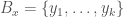
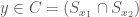
For reference, the nearest neighbor algorithm simply returns the vector within a dataset that has the smallest Euclidean distance from the input vector. Expressed symbolically, if $f(x,A)$ implements the nearest neighbor algorithm, as applied to $x$ , over $A$ , and $y = f(x,A)$ , for some $y \neq x$ , then $||x - y|| \leq ||x - z||$ , for all $z \in A$ . Further, assume that if there is at least one $y_i \in A$ , such that $||x - y|| = ||x - y_i||$ , then the nearest neighbor algorithm will return a set of outputs, $\{y, y_1, \ldots, y_k\}$ .

Lemma 1. If a dataset $A$ is locally consistent, then the nearest neighbor algorithm will never generate an error.

Proof. Assume that the nearest neighbor algorithm is applied to some dataset $A$ , and that $A$ is locally consistent. Further, assume that for some input vector $x$ , the output of the nearest neighbor algorithm, over $A$ , contains some vector $y$ , and that $y$ has a classifier that is not equal to the classifier of $x$ , thereby generating an error. Since $y$ is contained in the output of the nearest neighbor algorithm, as applied to $x$ , over $A$ , it follows that $||x - y||$ is the minimum over the entire dataset. Because $A$ is locally consistent, there is some nonempty set $B_x$ , that contains every vector $y_i$ , for which, $||x - y_i|| \leq \delta_x$ . Since $||x - y||$ is minimum, it must be the case that $||x - y|| \leq ||x - y_i|| \leq \delta_x$ , for all $y_i$ . But this implies that $y \in B_x$ , which contradicts our assumption that the classifiers of $x$ and $y$ are not equal. Therefore, if we nonetheless assume their classifiers are not equal, then $A$ is not locally consistent, which leads to a contradiction, thereby completing the proof.

What Lemma 1 says is that the nearest neighbor algorithm will never generate an error when applied to a locally consistent dataset, since the nearest neighbor of an input vector $x$ is always an element of $B_x$ , which guarantees accuracy. As a practical matter, if the nearest neighbor isn’t within $\delta_x$ of an input vector $x$ , then we can flag the prediction as possibly erroneous. This could of course happen when your training dataset is locally consistent, and your testing dataset adds new data that does not fit into any $B_x$ .

Corollary 2. A dataset is locally consistent if and only if the nearest neighbor algorithm does not generate any errors.

Proof. Lemma 1 shows that if a dataset $A$ is locally consistent, then the nearest neighbor algorithm will not generate any errors. So assume that the nearest neighbor algorithm generates no errors when applied to $A$ , and for each $x\in A$ , let $y_x$ denote a nearest neighbor of $x$ , and let $\delta_x = ||x - y_x||$ . Let $B_x = y_x$ , and so each $B_x$ is non-empty. If more than one vector is returned by the nearest neighbor algorithm for a given $x$ , then include all such vectors in $B_x$ . By definition, $||x - y_x|| \leq \delta_x$ . Therefore, there is a value $\delta_x > 0$ , for each $x\in A$ , such that the set of all points for which $||x - y_i|| \leq \delta_x$ , $B_x$ , has a single classifier, and $B_x$ is non-empty for all such $x$ , which completes the proof.

Corollary 3. A dataset is locally consistent around $x \in A$ , if and only if the nearest neighbor algorithm does not generate an error, when applied to $x$ , over $A$ .

Proof. Assume that the nearest neighbor algorithm does not generate an error when applied to $x \in A$ . It follows that there is some $B = \{y_1, \ldots, y_k\} \subseteq A$ , generated by the nearest neighbor algorithm, as applied to $x$ , over $A$ , for which $||x - y_i||$ is minimum, and the classifiers of $x$ and $y_i$ are all equal. Let $B_x = B$ , and let $\delta_x = ||x - y_i||$ . Since, the classifiers of $x$ and $y_i$ are all equal, this implies that $A$ is locally consistent around $x$ .

Now assume that $A$ is locally consistent around $x$ , and let $B = \{y_1, \ldots, y_k\} \subseteq A$ be the output of the nearest neighbor algorithm, as applied to $x$ , over $A$ . It follows that $||x - y_i||$ is minimum over $A$ , and therefore, $B \subseteq B_x$ . This implies that the classifier of $x$ equals the classifier of each $y_i$ , which completes the proof.

Clustering

We can analogize the idea of local consistency to geometry, which will create intuitive clusters that occupy some portion of Euclidean space. We say that a dataset $A$ is clustered consistently, if for every $x \in A$ , there exists some $\delta_x > 0$ , such that all points contained within a sphere of radius $\delta_x$ (including its boundary), with an origin of $x$ , denoted $S_x$ , have the same classifier as $x$ .

Lemma 4. A dataset is locally consistent if and only if it is clustered consistently.

Proof. Assume $A$ is locally consistent. It follows that for each $x \in A$ , there exists a non-empty set of vectors $B_x$ , each of which have the same classifier as $x$ . Moreover, for each $y_i \in B_x$ , it is the case that $||x - y_i|| \leq \delta_x$ . This implies that all vectors within $B_x$ are contained within a sphere of radius $\delta_x$ , with an origin of $x$ . Therefore, $A$ is clustered consistently.

Now assume that $A$ is clustered consistently. It follows that all of the vectors $y_i$ within $S_x$ have a distance of at most $\delta_x$ , from $x$ . Let $B_x$ be the set of all vectors within $S_x$ . This implies that for every $x \in A$ , there exists a non-empty set of vectors $B_x$ , all with the same classifier, such that for all $y_i \in B_x$ , $||x - y_i|| \leq \delta_x > 0$ . Therefore, $A$ is locally consistent, which completes the proof.

What Lemma 4 says, is that the notion of local consistency is equivalent to an intuitive geometric definition of a cluster that has a single classifier.

Lemma 5. If a dataset $A$ is locally consistent, and two vectors $x_1$ and $x_2$ have unequal classifiers, then there is no vector $y \in A$ , such that $y \in C = (S_{x_1} \cap S_{x_2})$ .

Proof. If the regions bounded by the spheres $S_{x_1}$ and $S_{x_2}$ do not overlap, then $C$ is empty, and therefore cannot contain any vectors at all. So assume instead that the regions bounded by the spheres $S_{x_1}$ and $S_{x_2}$ do overlap, and that therefore, $C$ is a non-empty set of points, and further, that there is some $y \in C$ , such that $y \in A$ .

There are three possibilities regarding the classifier of $y$ :

(1) It is equal to the classifier of $x_1$ ;

(2) It is equal to the classifier of $x_2$ ;

(3) It is not equal to the classifiers of $x_1$ or $x_2$ .

In all three cases, it follows that $y \in B_{x_1}$ , and $y \in B_{x_2}$ , which leads to a contradiction, since the Lemma assumes that the classifiers of $x_1$ and $x_2$ are not equal. Since these three cases cover all possible values for the classifier of $y$ , it must be the case that $y$ does not exist, which completes the proof.

What Lemma 5 says, is that if two clusters overlap as spheres, then their intersecting region contains no vectors from the dataset.

Corollary 6. If $A$ is locally consistent, then any clustering algorithm that finds the correct value of $\delta_x$ , for all $x \in A$ , can generate clusters over $A$ with no errors.

Proof. It follows immediately from Lemma 5, since any such algorithm could simply generate the sphere $S_x$ , for all $x \in A$ .

You can easily approximate the value of $\delta$ for every row in a dataset using the code I’ve attached below, as applied to the MNIST Fashion Dataset, and it also generates the set $B_x$ for every row (it’s stored in the “final_rows” in the attached code). You can then count how many rows are locally consistent, which allows you to measure the classification consistency of the dataset.

Here’s a more formal PDF document that presents the same results:

Analyzing Dataset Consistency Download

cmndline-2 Download

supervised_delta-1 Download

Vectorized Image Classification (RGB Version)

February 24, 2021February 25, 2021 / erdosfan / Leave a comment

Following up on my article from yesterday, here’s a full color version that can classify images using almost entirely vectorized processes, and the runtimes are excellent, though I’m still testing it, and going to apply it to a wider set of datasets –

As applied to a simple dataset I made up of three grocery items, a lime, an avocado, and a grapefruit (30 images total, 10 per class), it takes about 1/10 of one second to identify an item with perfect accuracy, which certainly makes it usable as a scanner at an actual grocery, though again, I’m going to test it more, and write a more formal article on the technique.

Below are three sample images, together with representative super-pixel images actually fed to the classifier algorithm.

Here’s the command line code:

2_24_21_cmdnline Download

Here’s the code that displays the super-pixel images:

cmndline-2_25_21 Download

Here’s the full image dataset.

Vectorized Nearest Neighbor

February 24, 2021 / erdosfan / Leave a comment

I’m working on an image classification algorithm, and I found an extraneous line of code in my nearest neighbor algorithm, which I’ve now reduced to eleven lines of code:

function nearest_neighbors = NN_fully_vectorized(dataset, N)
dataset = dataset(:,1:N); %removes the hidden classifier
num_rows = size(dataset,1);
temp_matrix = repmat(dataset’, [1 1 num_rows]);
ref_dataset = shiftdim(temp_matrix,2);
diff_matrix = sum((dataset.-ref_dataset).^2,2);
zero_indeces = 1:num_rows+1:num_rows*num_rows;
diff_matrix(zero_indeces) = Inf; %sets the zero entries to infinity
[a b] = min(diff_matrix);
nearest_neighbors = reshape(b,[num_rows 1]);
endfunction

Vectorized Image Preprocessing

February 23, 2021February 24, 2021 / erdosfan / Leave a comment

In a previous article, I introduced an algorithm that can quickly partition an image into rectangular regions, and calculate the average color in each region, which would then be used for image classification. When I applied it to the MNIST dataset, I got good results, but there was an apparent ceiling of about 87% accuracy that I couldn’t breach, regardless of how many rows of the dataset I used. My original MNIST preprocessing algorithm had much better results, and the prediction algorithm was the same, which suggests a question –

Why is this one not as good?

And I realized, the answer is, I didn’t get rid of the background of the image, which in the aggregate, ends up generating a significant amount of noise, because it’s not exactly the same in every image, yet it’s a substantial portion of each image, which cumulatively, interfered with the prediction algorithm.

As a solution, I simply nixed every dimension that has a standard deviation of less than the average standard deviation across all dimensions, by setting them to zero. What this says is, if a dimension doesn’t really move much across all rows in a dataset, in the context of image processing, it’s probably background. You can’t always say this is correct, but for the MNIST dataset, it’s obviously true, because the background is in roughly the same place in every image, and roughly equal in luminosity. This implies that the background dimensions should have significantly lower standard deviations than the average across all dimensions. And it turns out, this works quite well, and produces accuracy that is on par with my previous preprocessing algorithm (93.35%, given 2,500 rows). However, the difference is, in this case, this is a general approach that should work for all simple image datasets that have a roughly uniform background, unlike my previous preprocessing algorithm, which was specific to the MNIST dataset.

Information Overload

Uncategorized

You and I (Music)

A Note on Potential Energy

VeGa

VeGa – Updated Draft

Updated Deck / Library

Analyzing Classification Consistency

Vectorized Image Classification (RGB Version)

Vectorized Nearest Neighbor

Vectorized Image Preprocessing

Updated Summary of Software