The neutrino seems to be capable of the same type of indefinite movement in a vacuum that a photon is, and also apparently has a velocity of . However, the neutrino also appears to have mass, which suggests a gravitational field. None of these things are possible in relativity, yet experiments suggest, that this is how it is. This is however, perfectly fine in my model of physics, and in fact, I think I now have an elegant theory as to what’s going on in the neutrino.

In a note from earlier tonight, I postulated that the indefinite motion of a photon is due to a different state of the force carrier of gravity, that upon interaction with the photon, causes it to change position, indefinitely, at least when undisturbed in a vacuum. Similarly, a mass emits this same force carrier, in a different state, as the force carrier for gravity, that in turn changes the momentum of the particles with which it interacts.

So in the case of the neutrino, we have this same force carrier at work, changing the position of the neutrino, and being emitted, as the force carrier of gravity. There are no issues with conservation, because the force carrier of gravity cannot carry finite momentum anyway, since it cannot be exhausted or insulated against, so it doesn’t matter how many instances of this force carrier exist, so long as it’s not zero, which is distinct.

This also suggests the possibility of unstable neutrino-like particles, because my model implies that this force carrier could also change the state of a particle, not just its position (see Section 3 of this paper). Bizarrely, it also suggests the existence of a particle that is physically stationary, and never changes state, and is therefore literally stationary at a given moment in time, though nonetheless emits gravity (see Footnote 7 of “A Unified Model of the Gravitational, Electrostatic, and Magnetic Forces“, which implies that such a particle would have a velocity of zero in time).

Consider a truly stationary object, that also doesn’t change its properties, ever –

The object in question never moves, and never changes in anyway at all, though it exists, in that another system could cause it to accelerate.

Now consider time with respect to this object –

It simply doesn’t exist, in the absence of information about other systems, that are capable of change. As a consequence, if this system exists in a vacuum, in isolation, and is the only thing in the Universe, then there is no measurable time at all, since there is no measurable change.

Obviously, we don’t live in such a Universe, but it points to something fundamental, which is that time itself depends upon multiplicity of outcome –

If only one thing can happen, then time consists of only that one thing.

This in turn suggests that time is perhaps reasonably thought of as the set of all possible states of the Universe, in some connective order, that in turn defines what sequences of the Universe are physically possible.

In my model of physics, energy is quantized (see Section 2 of this paper), and moreover, energy is the fundamental underlying substance of all things. This gives photons real substance, since they’re comprised of nothing other than energy that happens to be moving. In contrast, mass is energy that happens to be stationary, in the absence of kinetic energy, which is simply light attached to mass, that causes the mass to move. This is obviously not inconsistent with Einstein’s celebrated mass-energy equivalence, but is instead more abstract, and includes and implies that mass and light are interchangeable and equivalent.

I also showed that from a set of assumptions that are completely unrelated to relativity, and that have nothing to do with time directly, and are instead rooted in combinatorics and information theory, you end up with the correct equations of physics, for everything, for time-dilation, gravity, charge, magnetism, and I’ve even tackled a significant amount of quantum mechanics as well (see this book, generally).

I spend most of my time now thinking about thermodynamics, and A.I., because the two are in my opinion deeply interconnected, and have commercial applications to drone technology, though I still think about theoretical physics, and in particular, the fact that light will apparently travel indefinitely in a vacuum. Related, in my opinion, is the fact that gravity cannot be insulated against. Both suggest an underlying mechanic that is inexhaustible, by nature. Moreover, mass-energy equivalence plainly demonstrates the connections between mass and light, which I think I’ve likely exhausted as a topic in the first paper I linked to above. However, I did not address the connections between the apparently perpetual nature of the motion of light in a vacuum, and the apparently inexhaustible acceleration provided by gravity.

I now think I have an explanation, which is as follows:

Whatever substance it is that allows for the indefinite motion of a photon is equivalent to the force carrier of gravity, though in a different state. Whatever this substance is, in the case of a photon, it is withheld by the photon, and in the case of mass, expelled by the mass, which we would therefore view as the force carrier of gravity.

This model effectively assumes that the force carrier of gravity also has two states, just like energy itself, which is either kinetic or massive. In the case of a photon, we have a force carrier that causes the photon itself to move, indefinitely. In the case of a mass, we have an expelled, independently moving force carrier for gravity, that causes unbounded acceleration in other systems (in that it cannot be insulated against or exhausted). In the jargon of my model, position is itself a code, as is what I call the “state” of a particle, which determines all of its properties. For example, the code for an electron is distinct from the code for a tau lepton (see Section 3 of this paper). This actually works quite well at the quantum level, where you have bosons that can literally change the properties of another particle altogether, which my model would view as an exchange of code, which is mathematically equivalent to momentum (see Equation 10 of this paper).

In this view, the gravitational force-carrier when acting on a photon changes the position code of the photon, indefinitely, causing it to move, indefinitely. Because code and momentum are equivalent in my model, this would be an exchange of momentum from the force carrier to the photon, that causes it to change position, which is, again, defined by a code. This view implies that the locomotive force of movement itself is due to this force carrier changing a code within the photon, which causes the appearance of motion over time. In the case of a mass emitting gravity, this force carrier would instead change the state of some exogenous particle, changing its properties, in this case its momentum and total energy.

There is a question of what happens to this force carrier, assuming it exists, when light travels through a medium –

Light certainly slows down in a medium, and light certainly changes behavior in some mediums, both of which suggest the possibility of perhaps separating light from whatever this force carrier is. If possible, then perhaps it could be applied to other systems, causing motion in those systems. Obviously, this would be a very valuable tool, if it exists, and further, assuming it can be separated from light, and further manipulated. Moreover, as a matter theory, it implies a conservation between mass and energy, in that mass emits gravity, whereas a photon does not, and this fills the gap.

You can quibble about this a bit, because the force carrier for gravity is emitted indefinitely, presumably separately, resulting in a large number of force carriers over time. In contrast, you arguably don’t need that to be the case to cause the position of a photon to change. However, because the accelerating power of gravity cannot be exhausted, gravity cannot cary finite momentum. Therefore, one such force carrier carries the same amount of momentum as any finite number of force carriers, and so, there is a conservation of momentum between the photon state of this carrier and the mass state of this carrier.

I already wrote an object tracking algorithm that is quite fast, however that algorithm uses spatial proximity between points to determine whether or not a group of points are all part of the same object. That is, if a set of points are sufficiently close together, then they’re treated as part of one object. Then, that object is tracked as it moves.

It just dawned on me that you could also track an object by looking at the motions of a set of points. For example, if you have two objects, one of which is stationary, the other of which is moving, then the point data for those objects will reflect this. You can calculate the velocity of the points by using the nearest neighbor method to map each point in frame 1 to a point in frame 2, and so on and so on (this is exactly how my earlier object tracking algorithm works). You could then look at the change in position between each frame, and assuming each frame is taken over a uniform amount of time, that change in position is equal to the velocity of the point.

You would then cluster the points using their velocities, which would cause in this case the points in the stationary object to be clustered together, since its points are not moving, and cause the points in the moving object to be clustered together, since they’re all moving at roughly the same velocity.

In a previous article, I introduced an efficient way to calculate spatial entropy, which is otherwise difficult to calculate (as far as I can tell). The main reason I use spatial entropy is to partition images, and so you can use this method to do exactly that, or more generally partition a space, by simply calculating the spatial entropy of your dataset first (just use method from my previous article, code below), which will be some value . Then, simply take the inverse log of , and take the floor or ceiling of that value. Note that the code I’ve attached automatically returns an integer value.  You can then use this number as the number of regions you partition your space into. So for example, if , then you would partition the space in question into equally sized regions, which would require regions per dimension, where is the dimension of the space in question.

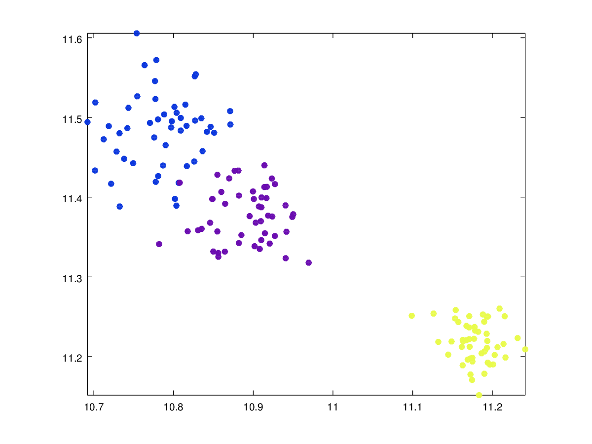
As it turns out, the original idea I had for visualizing datasets in the plane doesn’t quite work (as implemented literally), but after some minor tweaks, it actually works great (so far). I’ve included code that allows for display in either the plane or in three dimensions, but I think it’s much better to look at in the plane. The code itself generates all kinds of data that I didn’t unpack yet, that allows for answering questions like, which classes are the most similar in terms of their positions in their original Euclidean space. I’m going to add to the code below, to allow for more detailed analysis that includes these things like this, and I’m also going to apply it to more datasets, in particular the MNIST Datasets, in the hope that visually similar classes (e.g., ‘1’ and ‘7’) are mapped closer together than those that aren’t (e.g. ‘2’ and ‘6’).

This is a supervised algorithm, so I don’t think it has any substantive value for prediction or classification, but it’s useful because it allows you to get an intuitive sense of how classes are organized in the dataset, by visualizing the dataset in a two or three dimensional space.

As an example, above is the output of the algorithm as applied to the UCI Iris Dataset, which has three classes, embedded in the plane. The number of points in the plane equals the number of points in the dataset, and the number of points in each class equals the number of points in the underlying classes (each colored differently). Between classes in the embedding, (a) their relative distances and (b) spread, are determined by (a) the relative distances of the average vectors for each underlying class and (b) the standard deviations of each underlying class, respectively. Note that it is mathematically impossible to preserve the relative distances between points as a general matter, since we are reducing dimensions (e.g., there is no way to embed four equidistant points in the plane). But the gist is, you use Monte Carlo style evaluation to come up with a best-fit embedding in the plane or three-space, as applicable.

MATLAB CODE:

I just realized it’s probably more fair to report the error for my core clustering algorithm (not the others) differently than I do in my deck, while working on my embedding algorithm. I disclosed exactly how I calculate error, so it’s not a lie, but it’s not right, in the sense that even though the clusters are not mutually exclusive, the better answer is to say that the error is given as follows:

,

whereas in the deck, I say the error is given by,

.

The latter measure does capture something, in that the number of rows is the number of opportunities to make errors, but that’s not what you want in this context, which is the accuracy of the cluster itself, regardless of how many rows there are.

You can probably use A.I. to tune (A) the behavior of a physical system to (B) some other system which you are observing, using the environmental controls you have over (A). You would under this view let the machine figure out how to set the environmental controls over (A) to model the behavior of (B), given the analogous inputs, and a set of analogous measurements.

The rational path seems to be to give the machine an enormous set of measurements over both, and allow the machine to discover correlations on its own. This would require delivering simultaneous signals to both (A) and (B), and allowing the machine to discover these correlations. This will eventually allow the machine to discover what set of signals that control (A) correspond to analogous signals that control (B). You can then use this to figure out how to achieve a desired end state of (B) given (A), or more generally, model the behavior of (B), given (A), without in anyway disrupting the status of (B). This is a longwinded way of saying that we probably don’t need to test anything on human beings anymore, until we’re well into the realm of confidence in a particular solution, and in that case, you get their consent.

This could allow you to build a small model of a massive system, that behaves in a scaled manner.

I just came up with what I hope to be a great algorithm for visualizing datasets in the plane. Datasets typically have dimensions that exceed three-space, and often times are in the hundreds, if not thousands, which makes visualization difficult and likely arbitrary. Because you’re often starting with such a large dimension, you can’t be sure that such an embedding even exists in the plane. For example, just consider four equidistant points –

There’s no such thing in the plane, though you could of course have such a thing in four-dimensions, where you have a pyramid.

This implies that you necessarily have some error associated with any embedding of a dataset in the plane, but that’s fine, if what you’re trying to do is get a visual intuition for what your data actually looks like, in terms of how it’s arranged in its native space. The overall idea would be to preserve relative distances as closely possible, knowing that in some cases, it’s literally impossible to get it right, which is fine, because, again, this is a visualization tool, not an instrument of measurement.

So here’s the algorithm, which I’ll actually code tonight.

(1) Take all pairs of distances between the vectors in the dataset.

This step can be vectorized fully using my implementation of the nearest neighbor algorithm.

(2) Find the maximum distance between any two pairs of vectors among that set of all distances.

(3) Divide all such distances by that maximum, which will generate a set of distances over [0,1].

(4) Now generate random matrices of (x,y) pairs, one for each row of the dataset.

This step is trivial to vectorize in Matlab and Octave, simply create some number of pages of matrices as follows:

Test_Matrix = rand(num_rows, 2, num_simulations);

Where num_simulations is the number of pages, which is, plainly, the number of Monte Carlo simulations.

(5) Select the matrix of (x,y) pairs that produces distances that have the least error when compared to the related distances generated above in Step (3).

To be clear, the idea is to map each row of a given page in Test_Matrix, each of which is a matrix of dimension (num_rows, 2), to a row of the original dataset, which presumably has a much higher number of columns.

This can be implemented by running the nearest neighbor algorithm on each page of the Test_Matrix. This will produce a set of distances for each pair of (x,y) coordinates in that matrix. However, you will have to run the the nearest neighbor algorithm on each page in Test_Matrix individually, which will require a for loop, that has a number of iterations equal to num_simulations.

And that’s it, this is your best embedding, and obviously, the more simulations you can run, the better your embedding will be. You could of course also use this to visualize graphs on datasets, which could be particularly useful if you want to get a visual sense of connectivity among vectors in the dataset.

In a previous article, I showed that you can use the nearest neighbor algorithm to build a simple graph based upon which vectors in a dataset are nearest neighbors of one another. In simple terms, if two vectors are nearest neighbors, then you connect them with an edge. Once you do this for all vectors in the dataset, you will have a graph. It dawned on me earlier today that you can define a measure of dataset consistency by analyzing the properties of the resultant graph. Specifically, take the set of maximal paths in the dataset , and label the vertices with their classifiers. Now, for each such path in , simply take the entropy of the distribution of classifier labels. This is exactly the technique I introduced in another previous article, but I suppose I didn’t make it plain that it can apply to any dataset. You can also perhaps use this to measure whether any errors are due to truly similar classes by first converting the labels to measure-based classifiers, using the method I introduced in the article before this one. That is, if the errors only appear where two classes are truly similar, then maybe that’s the way it is and that’s the best you can do, or, you can somehow tighten your lens on the dataset, which is something you can actually do in my model of machine learning.

To be perfectly clear, if any given path in contains more than one classifier, then that path by definition implies that the nearest neighbor algorithm will generate an error, and therefore, the dataset is what I would call not locally consistent. Here’s a brief proof:

Assume that and are both vertices in some path within the set . Because they are both part of the same path, there must a subset of that connects to , which we’ll call . Assume that the classifier of is and that the classifier of is , for . It follows that as we traverse , beginning at , the classifiers of the vertices along that path must at some point change from to , and let be the edge where this change occurs. Note that it could be the case that . Because is the nearest neighbor of , and by definition the classifiers of and are unequal, it is the case that the nearest neighbor algorithm generated an error when given the input .