It just dawned on me you can construct a clean definition of a total wave, as a collection of individual waves, by simply stating their frequencies and their offsets from some initial position. For example, we can define a total wave T as a set of frequencies , and a set of positional offsets , where each is a proper frequency, and each is the distance from the starting point of the wave to where frequency first appears in the total wave. This would create a juxtaposition of waves, just like you find in an audio file. Then, you just need a device that translates this representation into the relevant sensory phenomena, such as a speaker that takes the frequencies and articulates them as an actual sound. The thing is, this is even cleaner than an uncompressed audio file, because there’s no averaging of the underlying frequencies –

You would instead define the pure, underlying tones individually, and then express them, physically on some device.

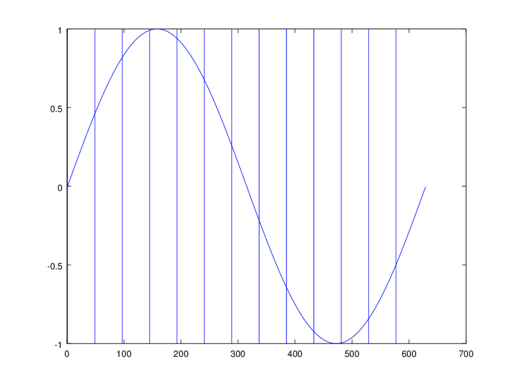
Revisiting the topic of periodicity, the first question I tried to answer is, given a point, how do you find the corresponding points in the following cycles of the wave? If for example, you have a simple sine wave, then this reduces to looking for subsequent points in the domain that have exactly the same range value. However, this is obviously not going to work if you have a complex wave, or if you have some noise.

You would be in this view looking for the straightest line possible across the range, parallel to the x-axis, that hits points in the wave, since those points will for a perfectly straight line, have exactly equal range values. So then the question becomes, using something like this approach, how do I compare two subsets of the wave, in the sense that, one could be better than the other, in that one more accurately captures some sub-frequency of the total wave. This would be a balancing act between the number of points captured, and the error between their respective values. For example, how do you compare two points that have exactly the same range value, and ten points that have some noise?

The Logarithm of a Vector

This led me to what is fairly described as vector entropy, in that it is a measure of diffusion that produces a vector quantity. And it seems plausible that maximizing this value will allow you to pull the best sets of independent waves from a total wave, though I’ve yet to test this hypothesis, so for now, I’ll just introduce the notion of vector entropy, which first requires defining the logarithm of a vector.

Defining the logarithm of a vector is straight forward, at least for this purpose:

If , then , and .

That is, raising to the power of the norm of produces the norm of , and both vectors point in the same direction. Note that because , and , it follows that .

This also implies a notion of bits as vectors, where the total amount of information is the norm of the vector, which is consistent with my work on the connections between length and information. It also implies that if you add two opposing vectors, the net information is zero. As a consequence, considering physics for a moment, two offsetting momentum vectors would carry no net momentum, and no net information, which is exactly how I describe wave interference.

Vector Entropy

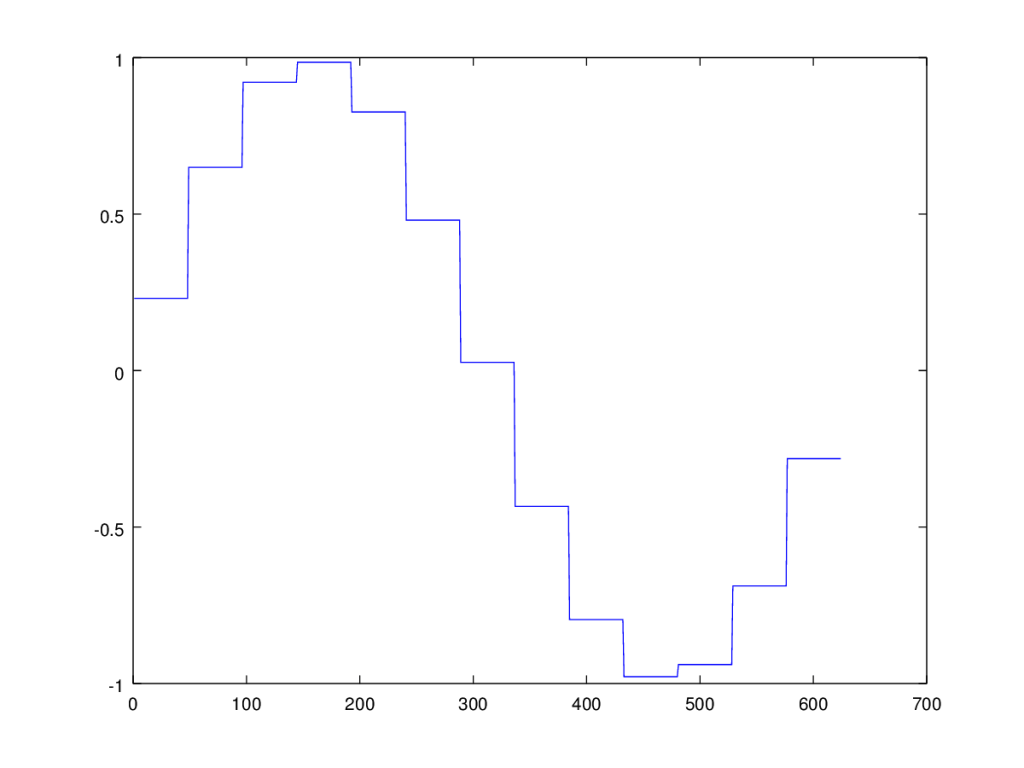
Now, simply read the wave from left to right (assuming a wave in the plane), and each point will define a vector, in order. Take the vector difference between each adjacent pair of vectors, and take the logarithm of that difference, as defined above. Then take the vector sum over the resultant set of difference vectors. This will produce a vector entropy, and the norm of that vector entropy is the relevant number of bits.

Expressed symbolically, we have,

Where has units of bits.

Lemma 1. The norm of is maximized when all are equal in magnitude and direction.

Proof. We begin by proving that,

is maximized when the norms of all are equal. Assume this is not the case, and so there is some . We can restate as,

Now let , and let . Note that if , then . Let us maximize , which will in turn maximize by taking the first derivative of , with respect to , which yields,

Setting to zero, we find , which in turn implies that has an extremal point when the arguments to the two logarithm functions are equal to each other. The second derivative is negative for any positive value of , and because is the sum of the norm of two vectors, is always positive, which implies that is maximized when . Since we assumed that is maximized for , we have a contradiction. And because this argument applies to any pair of vectors, it must be the case that all vectors have equal magnitudes.

For any set of vectors, the norm of the sum is maximized when all vectors point in the same direction, and taking the logarithm does not change the direction of the vector. Therefore, in order to maximize , it must be the case that all point in the same direction. Note that if all such vectors point in the same direction, then,

,

which completes the proof. □

Note that this is basically the same formula I presented in a previous note on spatial diffusion, though in this case, we have a vector quantity of entropy, which is, as far as I know, a novel idea, but these ideas have been around for decades, so it’s possible someone independently discovered the same idea.

In a previous article, I introduced an algorithm that can partition data observed over time, as an analog of my core image partitioning algorithm, which of course operates over space. I’ve refined the technique, and below is an additional algorithm that can partition a dataset (e.g., an audio wave file) given a fixed compression percentage, and it runs in about .5 seconds, per 1 second of audio (44100 Hz mono).

Here are the facts:

If you fix compression at about 90% of the original data, leaving a file of 10% of the original size, you get a decent sounding file, that visually plainly preserves the original structure of the underlying wave. Compression in this case takes about .5 seconds, per 1 second of underlying mono audio, which is close to real time (run on an iMac). If you want the algorithm to solve for “ideal” compression, then that takes about 1 minute, per 1 second of underlying mono audio, which is obviously not real time, but still not that bad.

The original wave

The compressed wave (98% compressed)

What’s interesting, is that not only is the audio quality pretty good, even when, e.g., compressing 98% of the underlying audio data, you also preserve the visual shape of the wave (see above). For a simple spoken audio dataset, my algorithm places the “ideal” compression percentage at around 98%, which is not keyed off of any normal notions of compression, because it’s not designed for humans, but is instead designed for a machine to be able to make sense of the actual underlying data, despite compression. So, even if you think the ostensibly ideal compression percentage sounds like shit, the reality is, you get a wave file that contains the basic structure of the original underlying wave, with radical compression, which i’ll admit, I’ve yet to really unpack and apply to any real tasks (e.g., speech recognition, which I’m just starting). However, if your algorithms (e.g., classification or prediction) work on the underlying wave file, then it is at least at this point not yet absurd that they would also work on the compressed wave, and that’s what basically all of my work in A.I. is based upon:

Compression for machines, not people.

And so, any function that turns on macroscopic structure, and not particulars, which is obviously the case for many tasks in A.I., like classification, can probably be informed by a dataset that makes use of far more compression than a human being would like. Moreover, if you have fixed capacity for parallel computing, then these types of algorithms allow you to take an underlying signal, and compress it radically, so that you can then generate multiple threads, so that you can, e.g., apply multiple experiments to the same compressed signal. Note that this is not yet fully vectorized, though it plainly can be, because it relies upon the calculation of independent averages. So even if, e.g., Octave doesn’t allow for full vectorization in this case, as a practical matter, you can definitely make it happen, because the calculations are independent.

Attached is the applicable code, together with a simple audio dataset of me counting in English.

Counting Dataset

My basic image partition algorithm partitions an image into rectangular regions that maximize the difference between the average colors of adjacent regions. The same can be done over time, for example, when given a wave file that contains audio, other amplitude data, or any time-series generally. And the reasoning is the same, in that minor changes in timing prevent row by row comparison of two sets of observations over time, just like noise in an image prevents pixel by pixel comparison in space, making averaging useful in both cases, since you group observations together, blurring any idiosyncrasies due to small changes in observation.

Below is the result of this process as applied to a simple sin wave in the plane, with the partitions generated by the algorithm on the left, and the resultant square wave produced by replacing each value with the average associated with the applicable region. Also attached is the Octave command line code.

Note that I made what is arguably a mathematical error in the function that partitions the time-series. Attached is a standalone function that accomplishes exactly this. Also attached is an algorithm that does the same given a fixed compression percentage.

In a previous article, I introduced a method that can quickly calculate spatial entropy, by turning distances in a dataset into a distribution over , that then of course has an entropy. This however does not vary with scale, in that if you multiply the entire dataset by a constant, the measure of entropy doesn’t change. Perhaps this is useful for some tasks, though it plainly does not capture the fact that two datasets could have the same proportional distances, but different absolute distances. If you want to measure spatial diffusion on absolute basis, then I believe the following could be a useful measure, that also has units of bits:

.

Read literally, you take the logarithm of every pair of distances within the dataset, which will of course vary as a function of those distances. As a result, if you scale a dataset up or down, the value of will change as a function of that scale. In a previous note, I showed that we can associate any length with an amount of information given by the logarithm of that length, and so we can fairly interpret as having units of bits.

Information, Length, and Volume

I’ve written about this topic a few times, and having reviewed it, the articulation was a bit sloppy, so I thought I’d restate it a bit more formally. The basic idea is that there’s some capacity for storage in each unit of length, and this is physically true, in that you can take a string, for example, and subdivide its length into equal intervals with markings. Then, simply place an object upon one of the markings –

This is a unique state of the system, and placing the object upon each other such marking defines a different unique state of the system.

If there are such markings, then the system can be in states, and therefore, store bits of information. This system is equivalent to a binary string of length , where only one bit can be flipped on at a time. We can generalize the connection between length and information by assuming that the length is divided into some number of segments, each of which can be in states. To continue with the physical intuition, this could be done by assigning objects to each of the segments along the length, where the number of objects placed upon a given segment determines its state. For example, if you have 2 pebbles upon a given marking along the string, that would be the second state of that segment. This generalization associates a given length with a -ary string of length , that can be in states, and store bits.

We can set a variable to have units of -ary switches per length, and so given a length , we can then solve for . The number of bits that can be stored along the length is therefore given by . Note that we can treat   and as constants as a function of , and as a result, the information content associated with a given length is . We can generalize this to volume, where would instead have units of -ary switches per volume, from which it follows that the information content associated with a given volume is also .

This in fact demonstrates that there is a proportional relationship between substance, and information. For an exhaustive treatment of this topic, my first real paper on physics implies an actual equation that relates energy and information (See Equation 10), and they are in that case again proportional. What the work above shows is that as a practical matter, at the macroscopic scale, the same proportional relationship holds, since my paper implies that the information content of a system is , where is the total energy of the system.

This is by far the meanest thing I have ever written, and is a plain parody of the tactics used by trusts in business, which are real, and always have been, except this time, the tech sector has unprecedented power. This is obviously also inspired by the Simpson’s Stone Cutters, and the Twig and Plum joke from 30 Rock.

successbookii

I’ve updated my deck yet again, to include supervised prediction, and of course to correct the mistakes I made in calculating error.

The code is here.

There’s some code floating around in my library (as of 6/21/21) that I never bothered to write about that generates a value of delta for each row in the dataset, independently, effectively implementing the ideas I go through in this paper on dataset consistency. What this means is, as a practical matter, you know how far you can go from a given point in the dataset, before you encounter your first inconsistent classification. For example, if is the vector for row i of the dataset, then the algorithm finds the distance , such that any sphere with a radius of , will contain a vector that has a class that is different from the class of . Obviously, you can use this to do supervised prediction, by simply using the nearest neighbor algorithm, and rejecting any predictions that match to row i, but are further away from than .

This is exactly what I did in my first set of A.I. algorithms, and it really improves accuracy. Specifically, using just 5,000 training rows from the MNIST Numerical dataset, this method achieves an accuracy of 99.971%, and it takes about 4 minutes to train. The downside, is that you reject a lot of predictions, but by definition, the rejected rows from the testing dataset are inconsistent with the training dataset. What this means as a practical matter, is that you need more data to fill the gaps in the training dataset, but the algorithm allows you to hit really high accuracies with not much data, and that’s the point of the algorithm. In this case, 30.080% of the testing rows were rejected. But the bottom line is, this obviously catches predictions that would have otherwise been errors.

I’ve updated my deck to clarify the way error is calculated (attached), and though it’s not much of a change, it’s certainly more precise now. There are links below to the same file on DropBox and ResearchGate as well.

IDropBox

IResearchGate