I’ve long suspected that the Phoenicians are the common ancestor of a lot of modern people in Northern Europe, parts of Africa, and East Asia. This is based on years of research at this point, but you can read this summary to get up to speed. I’ve finally developed a test that searches for the common maternal ancestor of the Tanzanians, the Basque, and the Koreans, and it turns out it’s still plausible that it’s the Phoenicians, but I’m starting to realize all of these tests simply tell me which population is the most ancient, without providing any obvious geography, which is what I’m really looking for. More to come, code below.
I started thinking about correlation again, and it dawned on me, that when we do math and science, we’re looking for computable relationships between sets of numbers. The most basic example is a function that describes the behavior of a system. Ideally, we have exact descriptions, but we often settle for probabilistic descriptions, or descriptions that are exact within some tolerance. I’d say that the search for computable relationships between sets of numbers is in fact science. But when you consider the full set of relationships between two sets of numbers, the set we’re interested in is therefore minuscule in terms of its density. In the extreme case, the set of computable functions has a density of zero compared to the set of non-computable functions. Yet, science and mathematics have come to the point where we can describe the behaviors of far away worlds, and nanoscopic terrestrial systems.
Therefore, it’s tempting to think that the computable is everything, and the balance of relationships are nonsense. For physical intuition, consider a Picasso painting represented as an RGB image, and compare that to the full set of random RGB images of the same size. What’s strange, is that the set in question will contain other known masterpieces, and new unknown masterpieces, if the image is large enough and the pixel size is small enough. And while I haven’t done the math, I’d wager the density of masterpieces is quite small, otherwise we’d all be famous painters, and since we’re not, I don’t think you can gamble your way into a masterpiece.
Similarly, if I have two sets of random numbers, and I simply connect them with strings, you’d probably think I’m a lunatic, though I’ve just defined a function. Whereas if I point out that I can inject the set of integers into the set of even integers, you’d swear I’m a genius. This might seem like unscientific thinking, but it isn’t. It’s arguably all the same, in that humans have a clear preference for computability, and that translates into a preference for symmetry over asymmetry. Personally, I listen to a lot of strange, highly random music, and enjoy Gregory Chaitin’s work as well, but in all seriousness, are we missing valuable information in the form of more complex functions, and perhaps tragically in the form of non-computable functions, assuming no non-computable machine exists?
I was again reading my absolute favorite book on mathematics, Mathematical Problems and Proofs [1] (no, I am not paid for this endorsement, it really is that great), and on page 11 of the text, Example 1.20 gives Euclid’s Theorem on Prime Numbers, demonstrating that the set of prime numbers must be infinite. I immediately recalled that all natural numbers are either prime, or the product of primes, known as the Fundamental Theorem of Arithmetic. This is a different result, the proof of which is not presented in [1] (at least I didn’t see it).
I checked Google, and there’s a straightforward proof using induction, but it lacks intuitive appeal. As such, I spent a few minutes this morning thinking about it, and I realized you can construct an intuitive proof. I haven’t seen this proof elsewhere, though it could be a known result. Even if it is known, what’s interesting is the structure of the proof, which is you can show that it must be the case that the algorithm upon which the proof relies, will eventually halt. This is pretty interesting, and maybe it’s a new form of proof. At a minimum, we have an intuitive proof of the Fundamental Theorem of Arithmetic that does not rely on induction.
The Proof
Assume you have a natural number . If is prime, then we’re done. So assume that is not prime. As such, it must be the case that , for , and therefore, . The intermediate result will be to show that all numbers are either prime, or have at least one prime factor, which we will then use to prove the Fundamental Theorem of Arithmetic. As such, if is prime, then we’re done. Therefore, assume is not prime, and as such, , for . We can of course continue to apply this process for increasing values of , generating decreasing values of . However, there are only finitely many numbers less than , and as such, this process must eventually terminate, producing a prime number . Note that , and as such, . Therefore, all natural numbers have at least one prime factor.
Now let’s express as the product of this prime number , and the remaining factors, , i.e., . Note that cannot be prime, so we can therefore run the algorithm above on , which will produce another prime number factor , and another remaining factor , such that . Note that it must be the case that , and in general, , and therefore it requires fewer steps to calculate each successive prime factor. Because the number of steps is always a natural number, this process must terminate. Therefore, will eventually be expressed as the product of a finite number of primes.
I’ve been thinking about the ability to model the Universe as a whole for about 10 years, and over the last few weeks, this thinking became rigorous, and today, I proved a formal result after reading my absolute favorite book on mathematics, Mathematical Problems and Proofs. Specifically, the text introduces Dedekind’s definition of an infinite set, which is that a set is infinite if it can be put into a one-to-one correspondence with one of its proper subsets. I then realized two things: (1) we can use Dedekind’s definition of infinity to ask whether a finite volume of space could contain a machine capable of predicting the behavior of the entire Universe and (2) that Dedekind’s definition of infinity is equivalent to an intuitive definition of infinity where a number is infinite if and only if it is greater than all natural numbers.
Predicting the Behavior of the Universe
Assume that we have a machine such that the output tape of contains the state of the Universe at time . That is, if we look at the output tape of at time , we will see a complete and accurate representation of the entire Universe at time , essentially predicting the future. It turns out we get very different answers depending upon whether we assume is within the Universe, or outside the Universe. This is plainly a thought experiment, but the case where is within the Universe is not, and has clear physical meaning, and so it is a serious inquiry. The plain conclusion is that we cannot realistically predict the behavior of the Universe as a whole, completely and accurately, absent what are unintuitive consequences discussed below.
Case 1: is within the Universe. Because the machine is within the Universe, it must be the case that the output tape for contains a complete and accurate representation of both the internal state of at time , and the output tape at time . We can represent this as , where is the state of the Universe excluding , is the internal state of , and is the output tape of .
However, , which means that the output tape at time given by , must also contain the output tape for . This recurrence relation does not end, and as a consequence, if we posit the existence of such a machine, the output tape will contain the entire future of the Universe. This implies the Universe is completely predetermined.
Case 2: is within the Universe, though is simply no longer required. Removing the requirement to represent the output tape is just to demonstrate that we still have a serious problem even in this case. Because we’re assuming the output tape does not need to contain a representation of its own output, this solves the recurrence problem, and so .
However, it must be the case that the total information on the output tape equals the total information in the Universe, since the output tape contains a complete and accurate representation of the Universe excluding the machine, and a complete and accurate representation of the internal state of the machine, which together is the entire Universe. Therefore, it must be the case that the Universe, and the output tape, which is within the Universe, must contain the same amount of information. Using Dedekind’s definition of infinity, it must be the case that the Universe and the machine contain an infinite amount of information. Because UTMs contain a finite amount of information, we are still stuck with a non-computable Universe.
Case 3: is outside the Universe, or the entire output tape is outside the Universe. In this case we can have a computable Universe that is in essence modeled or represented, respectively, by a copy of the Universe, that is housed outside of the Universe. Note that because in this case the output tape is always outside the Universe, it does not need to contain a representation of itself, solving the recurrence problem in Case 1. Further, because the output tape is outside the Universe, it can hold the same finite amount of information as the Universe, solving the Dedekind-infinite issue in Case 2.
The point is not that any of these cases are realistic, and instead, the point is that none of these cases are realistic, yet these are the only possible cases. The conclusion is therefore, that there doesn’t seem to be any clear path to a perfect model of the Universe, even if we have perfect physics.
Intuitive Infinity
Once I had completed the result above, I started thinking about infinity again, and I realized you can prove that a number is Dedekind infinite if and only if it is greater than all integers, which I call “intuitively infinite”. Dedekind infinity is great, and forces you to think about sets, but you also want to be sure that the idea comports with intuition, especially if you’re going to use the notion to derive physically meaningful results like we did above. Now this could be a known result, but I don’t see it mentioned anywhere saliently, and you’d think it would be, so since I’m frankly not interested in doing any diligence, here’s the proof.
Let’s start by saying a number is intuitively infinite if it is greater than all natural numbers. Now assume that and there is a one-to-correspondence . Further assume that the cardinality of , written , is not intuitively infinite, and as such, there is some , such that . Because is one-to-one, it must be the case that , but because , there must be some such that . Because , it must be the case that , but this contradicts the assumption that is one-to-one. Therefore, if and there is a one-to-correspondence , then is intuitively infinite.
Now assume that is intuitively infinite and further let be some singleton. It would suffice to show that , since that would imply that there is a one-to-one correspondence from to one of its proper subsets, namely . Assume instead that . It must be the case that , since you can show there is no smaller infinite cardinality. Because we have assumed that , then it must be the case that , since removing a singleton from a countable set does not change its cardinality. Note we are allowing for infinite numbers that are capable of diminution by removal of a singleton arguendo for purposes of the proof. Analogously, it must be the case , since assuming would again imply that adding a singleton to a countable set would change its cardinality, which is not true. As such, because , there must be some such that . That is, we can remove a subset from and produce a countable set .
As such, because , it must be the case that . However, on the lefthand side of the equation, the union over does not contribute anything to the total cardinality of , because is countable and is a singleton, whereas on the righthand side does contribute to the total cardinality because , which we’ve assumed to have a cardinality of less than . This implies that the number of elements contributed to an aggregation by union is not determined by the number of elements in the operand sets, and instead by the order in which we apply the union operator, which makes no sense. Therefore, we have a contradiction, and so , which completes the proof.
In a paper entitled, “A New Model of Computational Genomics” [1], I introduced an algorithmic test for ancestry using whole-genome mtDNA. I’ve since updated that test significantly, as described below. In this first of what will be a series of articles, I will present the results of this test as applied to specific regions of the world, in this case, to Scandinavia. Each of the articles will contain an independent summary of the algorithm and its overall results, and so you can read each independently.
Algorithmic Testing for Ancestry
Assume you’re given whole mtDNA genomes A, B, and C. The goal is to test whether genome A is the ancestor of both genomes B and C. It turns out, this is straight forward as a necessary (but not sufficient condition) for ancestry. Specifically, if we begin with genome A, and then posit that genomes B and C mutated independently away from genome A (e.g., groups B and C travelled to two distinct locations away from group A), then it is almost certainly the case that genomes B and C have fewer bases in common with each other, than they have in common with genome A.
For intuition, because we’ve assumed genomes B and C are mutating independently, the bases that mutate in each of B and C are analogous to two independent coins being tossed. Each mutation will reduce the number of bases in common with genome A. For example, if genome B mutates, then the number of bases that A and B have in common will be reduced. Note we are assuming genome A is static. Because B and C are mutating independently, it’s basically impossible for the number of bases in common between B and C to increase over time. Further, the rate of the decrease in common bases is almost certainly going to be higher between B and C, than between A and B, and A and C. For example, if there are 10 mutations in each of genomes B and C (i.e., a total of 20 mutations combined), then the match counts between A and B and A and C, will both decrease by exactly 10, whereas the match count between B and C should decrease by approximately 20. Let |AB| denote the match count between genomes A and B. We have then the following inequalities:
Case 1: If genome A is the common ancestor of both genomes B and C, then it is almost certainly the case that |AB| > |BC| and |AC| > |BC|. See, [1] for further details.
Even though this is only a necessary condition for ancestry, this pair of inequalities (coupled with a lot of research and other techniques), allowed me to put together a complete, and plausible, history of mankind [2], all the way back to the first humans in Africa.
Ancestry from Archaic Genomes
The simple insight I had, was that if A is not archaic, and B is archaic, then A can’t credibly be the ancestor of B. That is, you can’t plausibly argue that a modern human is the ancestor of some archaic human, absent compelling evidence. Further, it turns out the inequality (since it is a necessary but not sufficient condition) is also consistent with linear ancestry in two cases. Specifically, if |AB| > |BC| and |AC| > |BC|, then we can interpret this as consistent with –
Case 2: B is the ancestor of A, who is in turn the ancestor of C.
Case 3: C is the ancestor of A, who is in turn the ancestor of B.
If you plug in A = Phoenician, B = Heidelbergensis, and C = Ancient Egypt, you’ll find the inequality is satisfied for 100% of the applicable genomes in the dataset. Note that the dataset is linked to in [1]. It turns out you simply cannot tell what direction time is running given the genomes alone (unless there’s some trick I’ve missed), and so all of these claims are subject to falsification, just like science is generally. That said, if you read [2], you’ll see fairly compelling arguments consistent with common sense, that Heidelbergensis (which is an archaic human), is the ancestor of the Phoenicians, who are in turn the ancestors of the Ancient Egyptians. This is consistent with case (2) above.
Putting it all together, we have a powerful necessary condition that is consistent with ancestry, but not a sufficient condition, and it is therefore subject to falsification. However, one of these three cases is almost certainly true, if the inequalities are satisfied. The only question is which one, and as far as I can tell, you cannot determine which case is true, without exogenous information (e.g., Heidelbergensis is known to be at least 500,000 years old). You’ll note that cases (1), (2), and (3) together imply that A is always the ancestor of either B or C, or both. My initial mistake was to simply set B to an archaic genome, and assert that since A cannot credibly be the ancestor of B, it must be the case that A is the ancestor of C. Note that because A cannot credibly be the ancestor of B, Cases (1) and (3) are eliminated, leaving Case (2), which makes perfect sense: B is archaic, and is the ancestor of A, who is in turn the ancestor of C. However, this is not credible if C is also archaic, producing a lot of bad data.
Updated Ancestry Algorithm
The updated algorithm first tests literally every genome in the dataset, and asks whether it is at least a 60% match to an archaic genome, and if so, it treats that genome as archaic for purposes of the test, so that we avoid the problem highlighted above. This will allow us to reasonably assert that all tests involve exactly one archaic genome B, and therefore, we must be in Case (2). Interestingly, some archaic populations were certainly heterogenous, which is something I discussed previously. As a result, there are three ostensibly archaic genomes in the dataset, that do not match to any other archaic genomes in the dataset, and they are therefore, not treated as archaic, despite their archeological classification. You can fuss with this, but it’s just three genomes out of 664, and a total of 19,972,464 comparisons. So it’s possible it moved the needle in marginal cases, but the overall conclusions reached in [2] are plainly correct, given the data this new ancestry test produced.
There is however the problem that the dataset contains only Heidelbergensis, Denisovan, and Neanderthal genomes, leaving out e.g., Homo Erectus, and potentially other unknown archaic humans. There’s nothing we can do about this, since we’re constantly finding new archaic humans. For example, Denisovans were discovered in 2010, which is pretty recent, compared to Heidelbergensis, which was discovered in 1908. Moreover, the three genomes in question are possibly three new species, since they don’t match to Denisovan, Heidelbergensis, or Neanderthals. All of that said, taken as a whole, the results produced by this new algorithm, which makes perfect theoretical sense and must be true, are consistent with the results presented in [2]. Specifically, that humans began in Africa, somewhere around present day Cameroon, migrated to the Middle East, then Asia, producing the three most evolved maternal lines that I’ve identified, somewhere around Nepal, specifically, the Ancient Egyptians, the Vikings, and the Ancient Romans. The first two maternal lines are both found around the world, and descend from Heidelbergensis and Neanderthals and / or Denisovans, respectively, suggesting that many modern humans are a mix between the most evolved maternal lines that originated in three distinct archaic human populations, effectively creating hybrids. The Ancient Roman maternal line no longer exists, and seems to have been deliberately annihilated. For your reference, you can search for the Pre Roman Ancient Egyptian genome (row 320, which descends from Heidelbergensis) and the Icelandic genome (row 464, which descends from either Neanderthals or Denisovans, or both, it’s not clear).
Maternal Ancestry Among Scandinavians and Germans
Intuition suggests that the Sami People, who are indigenous Scandinavians, should as a general matter test as the ancestors of at least some Scandinavian people. At the same time, because all but the Finns and Sami speak Germanic languages, we would expect the Germans to test as the ancestors of at least some Scandinavian people. All of that said, during the Viking Age, the Scandinavians made use of a Phoenician-like alphabet, known as Runes, and so it’s at least possible we should see either Continental European ancestry (e.g., the Basque used similar scripts in antiquity), Middle Eastern ancestry, or some other form of ancestry that explains this otherwise anomalous alphabet. We will examine each of these questions below using the ancestry test.
Levänluhta
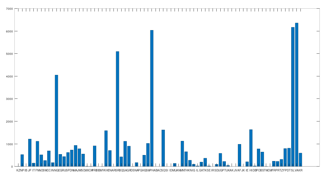
Levänluhta is an underwater gravesite in Finland that contains the remains of about 100 individuals from the Iron Age (c. 800 to 500 BC). Though Scandinavia has been occupied by humans since the Stone Age, common sense says that these individuals should test as the ancestor of at least some modern Scandinavians. This is indeed the case, and in fact, these individuals test as even more ancient than the Sami People, which you can see in the chart below. A positive number indicates that the population in question is a net ancestor, whereas a negative number indicates that the population in question is a net descendant. That is, if e.g., X is the number of times the ancestry test was satisfied from Sweden to Norway, and Y is the number of times the ancestry test was satisfied from Norway to Sweden, the chart below plots X – Y for each population. As you can see, all other Scandinavian groups test as the descendants of the individuals buried in Levänluhta. You can find the acronyms used below at the end of [1], but for now note that FN = Finland, NO = Norway, SW = Sweden, DN = Denmark, SM = Sami, IL = Iceland, and AF = Ancient Finland (i.e., Levänluhta). If you look at the ancestors of the individuals buried in Levänluhta (i.e., X – Y > 0), you’ll see HB = Heidelbergensis, AN = Andamanese, and other archaic populations, suggesting the individuals buried in Levänluhta are somewhere between archaic humans and modern humans, despite being a relatively recent Iron Age gravesite.
The Sami People
The Sami People are indigenous Scandinavians that speak an Uralic language and live in Northern Scandinavia, spanning Sweden, Norway, Finland, and Russia. For context, Uralic languages are spoken in regions around Finland, including Finland itself, Estonia, parts of Russia, as well Hungary. Uralic languages are to my knowledge not related to Germanic languages. As such, we should not be surprised if the Sami have a maternal ancestry that is distinct from the rest of the Scandinavians and Germans. This is in fact the case, and in particular, the Sami contain a significant amount of Denisovan mtDNA. See, [1] for more details. As noted above, Denisovans are a relatively recently discovered subspecies of archaic humans. The main archeological site where they were discovered is the Denisovan Cave in Siberia, and the dataset includes 8 Denisovan genomes from that site.
Above is the net maternal ancestry of the Sami people, where, again, a positive number indicates that the population in question is an ancestor of the Sami, and a negative number indicates that the population in question is a descendant of the Sami. As you can see above, all other living Scandinavian people test as the descendants of the Sami, making the Sami the most ancient among the living Scandinavian people.
The Finnish People
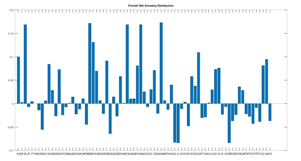
As noted above, the Finnish people speak an Uralic language, like the Sami, and as such, we should not be surprised if they have a distinct ancestry from the rest of the Scandinavians. This is in fact the case, though they are one step closer to modern Scandinavians than the Sami, and as you can see below, all Scandinavian people (other than the Sami) test as the descendants of the Finns.
Now this doesn’t mean that all the other Scandinavians descend directly from the Finns, which is too simple of a story, but it does mean that when comparing Finns to the rest of the Scandinavians (save for the Sami), it is more likely that a given Finn will test as the ancestor of a given Scandinavian, than the other way around. This is not terribly surprising since the Finns speak a completely different language that has (to my knowledge) an unknown origin, suggesting the language is quite ancient, and the Finns seem to be as well. The Finns also have a significant amount of Denisovan mtDNA from Siberia, which is again consistent with the claim that the Finns are, generally speaking, the second most ancient of the living Scandinavians.
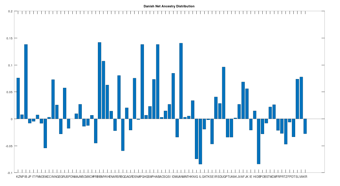
The Danish People
Like the Finns, the Danes also contain a significant but lesser amount of Siberian Denisovan mtDNA, and they similarly test as the ancestors of all other Scandinavians, other than the Finns and Sami, making them the third most ancient Scandinavian population. Note however that Danish is a Germanic language, suggesting independence between Uralic languages and Denisovan mtDNA, though there does seem to be some reasonable correlation.
The Norwegian People
The Norwegian people contain no meaningful quantity of Denisovan mtDNA, and they test as the fourth most ancient of the living Scandinavians. Note that the Sami, Finns, and Danes test as the net ancestors of the Norwegians, whereas the Swedes and Icelandic people test as the descendants of the Norwegians. Finally note that the Norwegians speak a Germanic language.
The Swedish People
The Swedes contain no meaningful quantity of Denisovan mtDNA, and they test as the fifth most ancient of the living Scandinavians, and are therefore more modern than the rest, save for the Icelandic (discussed below). The Swedes speak a Germanic language that is very similar to Norwegian, though the Swedes are notably distinct from the Norwegians in that they test as the descendants of the Germans, whereas the rest of the Scandinavians discussed thus far test as the ancestors of the Germans.
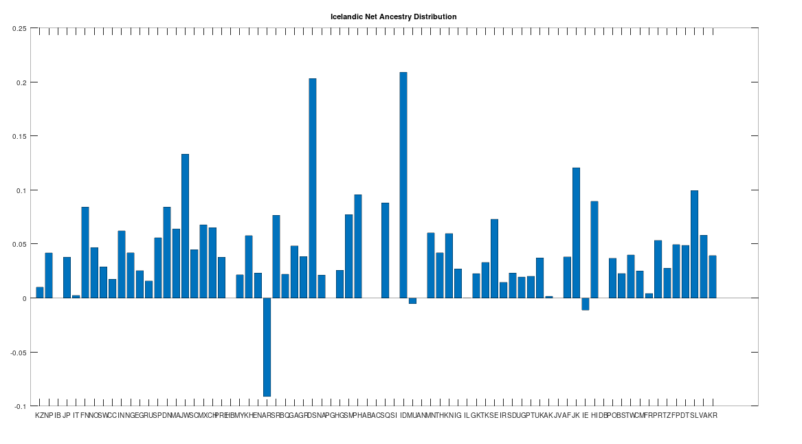
The Icelandic People
There is only one Icelandic genome in the dataset, but as you can see below, it is very similar to the Swedish population generally. Further, this genome tests as the descendant of all Scandinavian populations, and more generally, has only three descendants: the Ancient Romans, the Irish, and the Munda people of India. The Ancient Romans generally test as the descendants of the Northern Europeans, and are in fact the most modern population in the dataset according to this test. The Munda people of India are probably not Scandinavian, and instead, the Scandinavians and the Munda presumably have a common ancestor in Asia, consistent with the “Migration-Back Hypothesis” I presented in [2], that humanity begins in Africa, spreads to Asia, and then back to Northern Europe and Africa, as well as spreading into East Asia. Dublin was founded by the Vikings, so it is no surprise that some Irish test as the descendants of the Icelandic. However, there is only one Icelandic genome in the dataset, and so while we can’t say much about the Icelandic people in general on the basis of the dataset alone, because Iceland was (to my knowledge) uninhabited prior to the Vikings, it’s presumably the case that the people of Iceland are literally direct descendants of the Vikings, whereas in contrast, Scandinavia (as noted above) has been inhabited by humans since the Stone Age.
The Origins of the Runic Alphabet
Note that the Swedes and Icelandic are the only Scandinavians that test as a descendant as opposed to an ancestor of the Germans. This could explain why the majority of the Rune Stones are in Sweden, as opposed to the rest of Scandinavia. Specifically, the hypothesis is that Germanic people brought the Phoenician-like alphabet of the Runic Scripts to Sweden. As noted above, the Basque used a similar alphabet, who are also of course Continental Europeans, and so the overall hypothesis is that people of the Mediterranean (e.g., the Phoenicians themselves) brought their alphabet to the Continental Europeans, and the Germans brought that alphabet to the Swedes.
Asian and African Ancestors and Descendants of the Scandinavians
You’ll note in the charts above that some African and Asian people test as the ancestors and / or the descendants of the Scandinavians, in particular the Nigerians and Tanzanians, and the Koreans, Thai, and Japanese (though there are others). Though this might initially seem puzzling, it is instead perfectly consistent with the Migration-Back Hypothesis presented in [2], which asserts that many modern humans, in particular Northern Europeans, East Asians, and many Africans are the descendants of common ancestors from Asia.
The Ancient Mediterranean
The Ancient Romans are clearly descendants of the Northern Europeans, but I’ve found similar Italian genomes that are 35,000 years old. This implies that the most evolved genomes in the dataset are still at least 35,000 years old, and were already in Italy, long before Ancient Rome. The question is then, if the stage was set 35,000 years ago, in that the modern maternal lines were fully formed, why is that it took so long for civilization to develop? One possibility is that there was further evolution on the male line, or the rest of the genome, which is probably true given that mtDNA is, generally speaking, very slow to evolve.
However, civilization has geography to it, and it is simply impossible to ignore the Mediterranean, which produced the Ancient Egyptians, Mesopotamians, Ancient Greeks, and Ancient Romans, as well as others. Why did these people so drastically outperform literally all other humans? I think the answer is written language, and in turn, mathematics. That is, my hypothesis is that the genetics only gets you so far, and that you’ll find people very similar to e.g., the Phoenicians and Ancient Egyptians in other parts of the world that simply didn’t produce on the scale that the Mediterraneans did, and that the gap was driven by written language, which in turn allows for written mathematics, and everything that follows, from accurate inventories and contracts, to predictions about the future. That said, of all the Ancient and Classical people in the dataset, none of them contain any archaic mtDNA, suggesting maternal evolution really did play a role in intelligence and human progress.
This is difficult for modern people to appreciate, but imagine having no idea what happened a few weeks ago, and how that could leave you at a loss, or even put you at risk. At a minimum, written records reduce the risk of a dispute. Now imagine having no written system of mathematics, and trying to plan the construction of a structure, or travel over a long period of time. You’d have no means of calculating the number of days, or the number of individuals required, etc. Once you cross this milestone, it becomes rational to select mates on the basis of intelligence, which is a drastic shift from what happens in nature, which is selection for overall fitness. This seems to create a feedback loop, in that as civilizations become more sophisticated, intelligence becomes more important, further incentivizing selection for intelligence, thereby creating a more intelligent people.
This is not to diminish the accomplishments of other people, but it’s probably the case that the Mediterranean people of the Ancient and Classical periods were the most intelligent people in the world, at the time, which forces the question, of what happened to them? There’s unambiguous evidence that they were literally exterminated, at least in the case of the Romans. The thesis would therefore be that the Romans were slowly and systematically killed to the point of extinction, by less evolved people, creating the societal collapse and poverty that followed for nearly 1,000 years, until the Renaissance.
Unfortunately, it seems plausible the same thing is happening again. Specifically, consider that there have been no significant breakthroughs in physics since Relativity, which we now know is completely wrong. Also consider the fact that the most powerful algorithm in Machine Learning is from 1951. Not surprisingly, microprocessors have been designed using what is basically A.I., since the 1950s. So what is it then that these ostensible A.I. companies do all day? They don’t do anything, it’s impossible, because the topic began and ended in 1951, the only thing that’s changed, is that computers became more powerful. They are with certainty, misleading the public about how advanced A.I. really is, and it’s really strange, because scientists during the 1950s and 1960s, weren’t hiding anything at all. Obfuscation and dishonesty are consistent with a nefarious purpose, and companies like Facebook probably are criminal and even treasonous enterprises, working with our adversaries, and are certainly financed by backwards autocracies like Saudi Arabia.
If you’re too intelligent and educated, then you will know that the modern A.I. market is literally fake, creating an incentive to silence or even kill the most intelligent people, which is consistent with the extremely high suicide rate at MIT. It suggests the possibility that again, intelligent people are being exterminated, and having a look around at the world, it’s obvious that civilization is again declining, arguably when compared to the turn of the 20th Century, and certainly since the end of World War II. I think we all know who’s responsible, and it’s probably not Scandinavians.
Earlier this week I introduced a new ancestry algorithm, that is really incredible. It’s based upon a previous algorithm I introduced a few years back in a paper called “A New Model of Computational Genomics” [1]. The core difference between the new algorithm, and the algorithm introduced in [1], is that the algorithm introduced in [1] is a necessary but not sufficient condition for ancestry. This new algorithm, is instead a necessary and sufficient condition for ancestry, with a clearly identifiable risk, that is discussed in the note linked to above. Specifically, the risk is that the dataset only contains Denisovan, Heidelbergensis, and Neanderthal genomes, and as a consequence, because the test assumes it is considering exactly one archaic genome at a time, if it encounters e.g., Homo Erectus mtDNA, it won’t be able to identify it. Because the list of archaic humans keeps growing, this is a real and unavoidable risk, but as a whole, the algorithm clearly produces meaningful results. Most importantly, it produces results that are consistent with my “Migration Back Hypothesis” [2], that humanity began in Africa, migrated to the Middle East, then to Asia, and then came back to Europe and Africa, and spread further out from Asia into South East Asia.
The narrative is that life begins in Africa, somewhere around Cameroon, and this is consistent with the fact that the modern people of Cameroon test as the ancestors of Heidelbergensis, Neanderthals, and archaic Siberian Denisovans. See [2] for details. Heidelbergensis is clearly the ancestor of the Phoenicians, and you can run the test to see this, or read [2], where I actually analyze the Phoenician and Heidelbergensis genomes, segment by segment, demonstrating a clear ancestry relationship. The Phoenicians are in turn the ancestors of the Old Kingdom Ancient Egyptians, and this is where things get complicated.
The Old Kingdom Ancient Egyptians are obviously Asian, and this is based upon archeology, where depictions of Ancient Egyptian leaders and others are obviously of Asian origin, in particular Nefertiti. This checks out with the Old Kingdom Ancient Egyptian genome in the dataset, as it is a 99% match to many South East Asians in Thailand, Korea, and Japan in particular. The Phoenicians are clearly the maternal ancestors of the Ancient Egyptians, and so the question is, did the Phoenicians travel to Asia, eventually producing the Ancient Egyptian maternal line? The answer according to the new test is again yes, specifically, the modern Sardinians (who are basically identical to the Phoenicians) test as the ancestors of the modern Sri Lankan people. Previously, I did exactly this test in [2], and in that case, the Phoenicians again tested as the ancestors of the Sri Lankan people. The problem in [2], is that it was a low confidence answer, whereas the updated test provides a high confidence answer, drawn from the entire dataset of genomes. Finally, I’ll note that many modern Scandinavians and some other Europeans (typically in the North) are 99% matches to the Ancient Egyptian line. Putting it all together, humanity begins somewhere around Cameroon, migrates to the Middle East, and then migrates to Asia, where it then spreads back to Northern Europe and Africa, and spreads further into South East Asia. This is not different from the thesis presented in [2], but that thesis is now supported by a single test that draws on every genome in the dataset, creating clear scientific evidence for what was presented in [2] as a mix of archeological, scientific, and common sense reasoning.
In a previous post, I shared what I thought was a clever way of testing for ancestry, that turned out to be a failure empirically. I now understand why it doesn’t work, and it’s because I failed to consider an alternative hypothesis that is consistent with the purported facts. This produced a lot of bad data. I’ll begin by explaining how the underlying algorithmic test for ancestry works, and then explain why this instance of it failed, and close by introducing yet another test for ancestry that plainly works, and is simply amazing, allowing us to mechanically uncover the full history of mankind, using mtDNA alone.
Algorithmic Testing for Ancestry
Assume you’re given whole mtDNA genomes A, B, and C. The goal is to test whether genome A is the ancestor of both genomes B and C. It turns out, this is straight forward as a necessary (but not sufficient condition) for ancestry. Specifically, if we begin with genome A, and then posit that genomes B and C mutated independently away from genome A (e.g., groups B and C travelled to two distinct locations away from group A), then it is almost certainly the case that genomes B and C have fewer bases in common with each other, than they have in common with genome A.
For intuition, because we’ve assumed genomes B and C are mutating independently, the bases that mutate in each of B and C are analogous to two independent coins being tossed. Each mutation will reduce the number of bases in common with genome A. For example, if genome B mutates, then the number of bases that A and B have in common will be reduced. Note we are assuming genome A is static. Because B and C are mutating independently, it’s basically impossible for the number of bases in common between B and C to increase over time. Further, the rate of the decrease in common bases is almost certainly going to be higher between B and C, than between A and B, and A and C. For example, if there are 10 mutations in each of genomes B and C (i.e., a total of 20 mutations combined), then the match counts between A and B and A and C, will both decrease by exactly 10, whereas the match count between B and C should decrease by approximately 20. Let |AB| denote the match count between genomes A and B. We have then the following inequalities:
Case 1: If genome A is the common ancestor of both genomes B and C, then it is almost certainly the case that |AB| > |BC| and |AC| > |BC|. See, “A New Model of Computational Genomics” [1] for further details.
Even though this is only a necessary condition for ancestry, this pair of inequalities (coupled with a lot of research and other techniques), allowed me to put together a complete, and plausible, history of mankind [2], all the way back to the first humans in Africa.
Ancestry from Archaic Genomes
The simple insight I had, was that if A is not archaic, and B is archaic, then A can’t credibly be the ancestor of B. That is, you can’t plausibly argue that a modern human is the ancestor of some archaic human, absent compelling evidence. Further, it turns out the inequality (since it is a necessary but not sufficient condition) is also consistent with linear ancestry in two cases. Specifically, if |AB| > |BC| and |AC| > |BC|, then we can interpret this as consistent with –
Case 2: B is the ancestor of A, who is in turn the ancestor of C.
Case 3: C is the ancestor of A, who is in turn the ancestor of B.
If you plug in A = Phoenician, B = Heidelbergensis, and C = Ancient Egypt, you’ll find the inequality is satisfied for 100% of the applicable genomes in the dataset. Note that the dataset is linked to in [1]. It turns out you simply cannot tell what direction time is running given the genomes alone (unless there’s some trick I’ve missed), and so all of these claims are subject to falsification, just like science is generally. That said, if you read [2], you’ll see fairly compelling arguments consistent with common sense, that Heidelbergensis (which is an archaic human), is the ancestor of the Phoenicians, who are in turn the ancestors of the Ancient Egyptians. This is consistent with case (2) above.
Putting it all together, we have a powerful necessary condition that is consistent with ancestry, but not a sufficient condition, and it is therefore subject to falsification. However, one of these three cases is almost certainly true, if the inequalities are satisfied. The only question is which one, and as far as I can tell, you cannot determine which case is true, without exogenous information (e.g., Heidelbergensis is known to be at least 500,000 years old). You’ll note that cases (1), (2), and (3) together imply that A is always the ancestor of either B or C, or both. My initial mistake was to simply set B to an archaic genome, and assert that since A cannot credibly be the ancestor of B, it must be the case that A is the ancestor of C. Note that because A cannot credibly be the ancestor of B, Cases (1) and (3) are eliminated, leaving Case (2), which makes perfect sense: B is archaic, and is the ancestor of A, who is in turn the ancestor of C. However, this is not credible if C is also archaic, producing a lot of bad data.
Updated Ancestry Algorithm
The updated algorithm first tests literally every genome in the dataset, and asks whether it is at least a 60% match to an archaic genome, and if so, it treats that genome as archaic for purposes of the test, so that we avoid the problem highlighted above. This will allow us to reasonably assert that all tests involve exactly one archaic genome B, and therefore, we must be in Case (2). Interestingly, some archaic populations were certainly heterogenous, which is something I discussed previously. As a result, there are three ostensibly archaic genomes, that do not match to any other archaic genomes in the dataset, and they are therefore, not treated as archaic, despite their archeological classification. You can fuss with this, but it’s just three genomes out of 664, and a total of 19,972,464 comparisons. So it’s possible it moved the needle in marginal cases, but the overall conclusions reached in [2] are plainly correct, given the data this new ancestry test produced.
There is however the problem that the dataset contains only Heidelbergensis, Denisovan, and Neanderthal genomes, leaving out e.g., Homo Erectus, and potentially other unknown archaic humans. There’s nothing we can do about this, since we’re constantly finding new archaic humans. For example, Denisovans were discovered in 2010, which is pretty recent, compared to Heidelbergensis, which was discovered in 1908. Moreover, the three genomes in question are possibly three new species, since they don’t match to Denisovan, Heidelbergensis, or Neanderthals. All of that said, taken as a whole, the results produced by this new algorithm, which makes perfect theoretical sense and must be true, are consistent with the results presented in [2]. Specifically, that humans began in Africa, somewhere around present day Cameroon, migrated to the Middle East, then Asia, producing the two most evolved maternal lines that I’ve identified, somewhere around Nepal. Those two maternal lines are both found around the world, and descend from Denisovans and Heidelbergensis, respectively, suggesting that many modern humans are a mix between the most evolved maternal lines that originated in two distinct archaic human populations, effectively creating hybrids. For your reference, you can search for the Pre Roman Ancient Egyptian genome (row 320, which descends from Heidelbergensis) and the Icelandic genome (row 464, which descends from Denisovans).
The Distribution of Archaic mtDNA
When I first started studying mtDNA, I quickly realized that a lot of modern humans have archaic mtDNA. See [1] for details. This is not surprising, since mtDNA is so stable, and inherited directly from a mother to its offspring, and modern humans carry at times significant quantities of archaic DNA generally. That said, 53.01% of the genomes in the dataset test as archaic, meaning that the genome is a few hundred thousand years old, without that much change. I’ve seen studies that say some humans contain around 7% to 10% archaic DNA (on the high end). This is not exactly the same statement, since those types of studies say that around 7% to 10% of someone’s DNA could be archaic. In contrast, my work suggests that a significant majority of living human beings contain outright archaic mtDNA.
That said, I’m using whole-genome sequencing, with a single global alignment, which maximizes the differences between genomes. See [2] for more details. So it’s possible that as techniques improve, studies in other areas of the human genome will produce results similar to mine, since most researchers are (as far as I know) still focusing on genes, which are a tiny portion of the whole genome. Generally speaking, my work shows that focusing on genes is probably a mistake, that was driven by necessity since genomes are huge, and computers were slow. See [1] for empirical results that demonstrate the superiority of whole-genome analysis. I did all of this on a Mac Mini, and it runs in about 3 hours, and requires comparing all triplets of genomes, drawn from a dataset of 664 genomes (i.e., rows), where each genome has 16,579 bases (i.e., columns). This works out to calculations, all done on a consumer device. I’d wager professional computers can now start to tackle much larger genomes using similar techniques. As a result, I think we’re going to find that a lot of people contain a lot of truly archaic DNA generally. Any argument to the contrary is sort of strange, because if people stopped selecting archaic female mates, then archaic mtDNA should have vanished, and it obviously didn’t, leading to the conclusion, that the rest of the genome likely does contain archaic DNA generally.
Below I’ve set out a list of populations ordered according to the percentage of genomes within that population that test as archaic, starting at 0% archaic, and increasing up to 100% archaic, i.e., in increasing order. The test performed was to ask, for each population, what percentage of the genomes in that population are at least a 60% match to at least one archaic genome. Again, 53.01% of the full dataset tested as archaic, and as you’ll see below, several modern populations consist of only archaic mtDNA (i.e., 100% of the genomes are a 60% match to at least one archaic genome). One immediate takeaway, is that the classical world seems to have absolutely no archaic mtDNA. I’ve also noted that the Ancient Roman maternal line seems to have been annihilated, which was almost certainly deliberate.
Finally, I’ll note that preliminary results suggest that the Ancient Roman maternal line (which again, no longer exists, anywhere in the world) seems to be the most evolved maternal line in the entire dataset.
The code is attached to the bottom of the post.
0% Archaic
Ancient Egyptian Ancient Roman Basque Phoenecian Saqqaq Thai Igbo Icelandic Hawaiin Dublin Sri Lanka
10% to 49% archaic
Polish Sardinian Tanzania Korean German Swedish Scottish Nepalese Japanese Sami Filipino Dutch Spanish Sephardic Belarus Norwegian Egyptian Finnish Pashtun Ukrainian Irish French Portuguese Danish English
50% to 99% Archaic
Chinese Maritime Archaic Georgian Munda Nigerian Ashkenazi Mongolian Hungarian Ancient Finnish Greek Russian Mexican Vedda Abor. Italian Turkish Chachapoya Khoisan Neanderthal Uyghur Kenyan Indian Saudi Kazakh Denisovan Mayan Taiwanese
100% Archaic
Iberian Roma Heidelbergensis Papau New Guinea Ancient Bulgarian Ancient Chinese Sol. Islands Indonesian Andamanese Iranian Ancient Khoisan Javanese Jarkhand Cameroon
In a paper I wrote entitled A New Model of Computational Genomics [1], I presented a simple test for ancestry that is impossible to argue with. Let |AB| denote the number of matching bases between two genomes A and B. Given genomes A, B, and C, if we assume that genome A is the common ancestor of genomes B and C, then it is almost certainly the case (see [1] for a discussion of the probabilities) that |AB| > |BC| and |AC| > |BC|. That is, genomes A and B, and A and C, almost certainly have more bases in common than genomes B and C. For intuition, beginning with genome A, and assuming independent mutations away from A to genomes B and C, this is like tossing two independent coins (i.e., the mutations within genomes B and C that deviate from A), which should not have more than chance in common. As such, B and C should deviate away from each other at a faster rate than they deviate from A individually.
Now this is already really powerful, and led me to a complete history of mankind, which is more than plausible. But that said, it’s a necessary condition, not a sufficient condition. That is, if genome A is the common ancestor of genomes B and C, then the inequalities above almost certainly hold, but it’s subject to falsification (i.e., it’s not a sufficient condition). I realized tonight, you can actually transform this into a necessary and sufficient condition.
Specifically, the inequality above can be represented as a graph where A is connected to B, A is connected to C, and B is connected to C, with the match counts labelling the edges of the graph. For example, the edge connected A to B would be labeled with |AB|, which will be some integer. If the inequalities are satisfied, only two such graphs out of six are plausible, for the same reasons that underly the inequality. Specially, if I assume A is the ancestor of B, which is in turn the ancestor of C, then A and C almost certainly have fewer bases in common than A and B.
The graphs that remain, imply that if the inequality is satisfied, then A is almost certainly the ancestor of either B or C, or both, as a necessary and sufficient condition. If we plug in an implausible genome for either B or C (e.g., assuming that the Norwegians = A are the ancestors of Heidelbergensis = B), then the inequality serves as a necessary and sufficient condition for the descendants of the Norwegians, i.e., genome C. I will write more about this tomorrow, including code and some testing.
UPDATE 10/19/25
I’ve implemented a new version of the ancestry algorithm, which so far seems to work. Code is attached below, more to come!
I spend a lot of time thinking about the connections between information theory and reality, and this led me to both a mathematical theory of epistemology and a completely new model of physics. I did work on related foundations of mathematics in Sweden back in 2019, but I tabled it, because the rest of the work was panning out incredibly well, and I was writing a large number of useful research notes. Frankly, I didn’t get very far in pure mathematics, other than discovering a new number related to Cantor’s infinite cardinals, which is a big deal and solves the continuum hypothesis, but short of that, I produced basically nothing useful.
Euler’s Identify is False
Recently I’ve had some more free time, and I started thinking about complex numbers again, in particular Euler’s Identity. I’m a graph theorist “by trade”, so I’m not keen on disrespecting what I believe to be a great mathematician, but Euler’s identity is just false. It asserts the following:
.
I remember learning this in college and thinking it was a simply astonishing fact of mathematics, you have all these famous numbers connected through a simple equation. But iconoclast that I am, I started questioning it, specifically, setting , which implies that,
, and therefore,
, and so .
This implies that,
, and therefore, .
Now typically, we assume that . However, applying this produces a contradiction, specifically, we find that,
, which implies that , and therefore .
This implies that , which contradicts the assumption that . That is, the exponent of that produces 1 cannot be 0, since we’ve shown that . Therefore, we have a contradiction, and so Euler’s identity must be false, if we assume .
A New Foundation of Mathematics
I proved the result above about a week ago, but I let it sit on the back burner, because I don’t want to throw Euler, and possibly all complex numbers, under the bus, unless I have a solution. Now I have a solution, and it’s connected to a new theory of mathematics rooted in information theory and what I call “natural units”.
Specifically, given a set of binary switches, the number of possible states is given by . That is, if we count all possible combinations of the set of switches, we find it is given by 2 raised to the power of the cardinality of the set. This creates a connection between the units of information, and cardinality. Let’s assume base 2 logarithms going forward. Specifically, if is a set, we assume the cardinality of , written , has units of cardinality or number, and has units of bits. Though otherwise not relevant at the moment (i.e., there could be deeper connections), Shannon’s equation for Entropy also implies that the logarithm of a probability has units of bits. Numbers are generally treated as dimensionless, and so are probabilities, again implying that the logarithm always yields bits as its output.
The question becomes then, what value should we assign to ? Physically, a system with one state cannot be used to meaningfully store information, since it cannot change states, and as such, the assumption that has intuitive appeal. I’m not aware of any contradictions that follow from assuming that (other than Euler’s identity), so I don’t think there’s anything wrong with it, though this of course doesn’t rule out some deeply hidden contradiction that follows.
However, I’ve discovered that assuming implies true results. Physically, the assertion that is stating that, despite not having the ability to store information, a system with one state still carries some non-zero quantity of information, in the sense that it exists. As we’ll see, cannot be a real number, and has really unusual properties that nonetheless imply correct conclusions of mathematics.
If we assume that , it must be the case that . We can make sense of this by assuming that is defined over , other than at , where it is simply undefined. This makes physically intuitive sense, since you cannot apply an operator a zero number of times, and expect a non-zero answer, at least physically. To do something zero times is to do literally nothing, and so the result must be whatever you started with, which is not exactly zero, but it cannot produce change. Now you could argue I’ve just made up a new number, but so what? That’s precisely the point, because it’s more physically intuitive than standard axioms, and as we’ll show, it implies true results. Further, interestingly, it implies the possibility that all of these numbers are physically real (i.e., negative and complex numbers), though they don’t have any clear expression in Euclidean 3-space (e.g., even credits and debits are arguably better represented as positive magnitudes that have two directions). That is, the assumption is that things that exist always carry information, which is not absurd, physically, and somehow, it implies true results of mathematics.
Again, , and so , which implies that , and as such, . If we consider , we will find two correct results, depending how we evaluate the expression. If we evaluate what’s under the radical first, we have . If however we evaluate , we instead have , which is also correct. I am not aware of any number that behaves this way, producing two path-dependent but correct arithmetic results. Finally, because , it follows that , and so , where .
As a general matter, given , we have . Exponentiating, we find , but it suggests that is an iterator, that gives numbers physical units, in that is not dimensionless, though it is unitary.
This is clearly not a real number, and I’m frankly not sure what it is, but it implies true results, though I am in no position to prove that it implies a consistent theory of arithmetic, so this is just the beginning of what I hope will be a complete and consistent theory of mathematics, in so far as is possible, fully aware that the set of theorems on integers is uncountable, whereas the set of proofs is countable.
Information, Fractional Cardinals, Negative Cardinals, and Complex Cardinals
The fundamental idea is that a system will have some quantity of information that can be known about the system, and so everything I know about the system plus what I don’t know about the system must equal what can be known about the system. Specifically, we assume that , where is the set of states of the system in question. This turns out to be empirically true, and you can read the paper to learn more. Specifically, I present two methods for rigorously calculating the values and , one is combinatorial, and the other is to use Shannon’s entropy equation for . The results clearly demonstrate the equation works in practice, in addition to being philosophically unavoidable.
Because will have units of bits, and must also have units of bits. Therefore, we can exponentiate the equation using sets and , producing the following:
, where , , and .
Even if we restrict to integer cardinalities, which makes perfect sense because it is the number of states the system in question can occupy, it is possible for either of and to have a rational number cardinality. The argument is, exponentiating by some number of bits produces cardinalities. Because both and have units of bits, regardless of their values, if we assume the relationship between information and number holds generally, it must be the case that there are cardinalities and . Because either could be a rational number, we must accept that rational cardinalities exist, given that the equation is true, both empirically and philosophically. The same is true of negative cardinalities and complex cardinalities given the arguments above regarding , though there seems to be an important distinction, which is discussed below.
Inconsistency between Assumptions Regarding the Logarithm
It just dawned on me, after writing the article, that the discussion above presents what seem to be two independent, and inconsistent axioms regarding the logarithm. Specifically, the exponentiated equation requires that . As an example, let’s assume we’re considering a set of boxes, one of which contains a pebble, and we’re interested in the location of the pebble. As described, this system has possible states (i.e., locations of the pebble) and, therefore .
Now assume you’re told (with certainty) that the pebble is not in the first box. You are now considering a system with possible states, and so your uncertainty has been reduced. However, because this information doesn’t change the underlying system in any way, and in general, cannot change as a result of our knowledge of the system, it must be the case that your Knowledge is given by , which is non-zero. We can then reasonably assume that contains states, and that . Now assume you’re told that all but one box has been eliminated as a possible location for the pebble. It follows that , and that . If is not zero, fails. Because it is a tautology, and empirically true, it must be the case that , which is plainly not consistent with the arguments above regarding .
Now you could say is a bunch of garbage, and that’s why we have already found a contradiction, but I think that’s lazy. I think the better answer is that governs representations, not physical systems, and is only true with regards to representations of physical systems. We can then conclude that applies only to representations of physical systems, as an idea. Because is rooted in a physically plausible theory of the logarithm, we can say that this other notion of the logarithm governs physical systems, but does not govern representations of physical systems, since it clearly leads to a contradiction.
The question is then, as a matter of pure mathematics, are these two systems independent? If so, then we have something like the Paris Harrington Theorem. At the risk of oversimplification, the idea is that the mathematics that governs our reality in Euclidean 3-space could be different than the Platonic mathematics that governs representations, or perhaps ideas generally.
I’ll note that is a subjective measure of information related to a representation of a system, in that while is an objective invariant of a system, and are amounts of information held by a single observer. In contrast, is rooted in the physically plausible argument that if a thing exists in Euclidean 3-space (i.e., it has some measurable quantity), then it must carry information, even if it is otherwise static in all other regards.
Interestingly, if we accept the path-dependent evaluation of , and we believe that is the result of a physically meaningful definition of the logarithm, then this could provide a mathematical basis for non-determinism, in that physical systems governed by (which is presumably everything, if we accept that all extant objects carry information), allow for more than one solution, mechanically, in at least some cases. And even if it’s not true non-determinism, if we view 1 in the sense of being the minimum amount of energy possible, then is definitely a very small amount of information, which would create the appearance of non-determinism from our scale of observation, in that the order of interactions would change the outcomes drastically, from -1 to 1.
In closing, I’ll add that in the exponentiated form, , neither set can ever be empty, otherwise we have an empty set , which makes no sense, because again, the set can’t change given our knowledge about the set. Once we have eliminated all impossible states, will contain exactly one element, and will contain all other elements, which is fine. The problem is therefore when we begin with no knowledge, in which case , in the sense that all states are possible, and so our uncertainty is maximized, and our knowledge should be zero. However, if is empty, then we have no definition of .
We instead assume that begins non-empty, ex ante, in that it contains the cardinality of , which must be known to us. Once our knowledge is complete, will contain all impossible states of , which will be exactly in number, in addition to the cardinality of , which was known ex ante, leaving one state in , preserving the tautology of both and .
I noticed a while back that individual subspecies of archaic humans were actually heterogenous, at least with regards to their mtDNA. In particular, the Neanderthal genomes in my dataset are actually 6 completely different maternal lines. There are 10 Neanderthal genomes in total, and the breakdown is (i) genomes 1, 2, and 10 are at least a 99.5% mutual match to each other, (ii) genomes 5 and 6 are a 63.4% match to each other, (iii) genomes 8 and 9 are a 99.9% match to each other, and (iv) genomes 3, 4, and 7 are unique, and have no meaningful match to each other or the rest of the Neanderthal genomes. Further, clusters (i), (ii), and (iii) have no meaningful match to each other. The plain result is that we actually have a heterogenous group of genomes, that have nonetheless been classified as Neanderthal.
Now I’m in no position to criticize archaeological work, but you can’t ignore the fact that we have 6 completely distinct classes of genomes. Because, by definition, there must be 6 distinct maternal lines in this population, it’s probably the case that the rest of the genome also differs meaningfully, though note the number of paternal lines could be larger or smaller than 6. But the point remains, the genomes probably differ generally, not just along the maternal line.
As a result, we have to ask whether we actually have a single subspecies. If we take that view, then the subspecies is the result of the mixing of these 6 distinct maternal lines. And this makes perfect sense, because the vast majority of human populations have heterogeneous maternal lines, and the only exceptions I’m aware of are the Romani People and the Papuans, who are almost perfectly homogenous on the maternal line. It’s worth noting that Romani mtDNA is basically identical to Papuan mtDNA, so there’s probably something to that.
We could instead take the view that the archeological classification is wrong, and that mtDNA controls the definition of a subspecies. I think this is a little aggressive, given that mtDNA is a very small portion of the overall human genome. But at the same time, mtDNA conveys a lot of information about heredity and even conveys information about paternal ancestry, which is amazing. That said, I think the better view is that a given group of people is (generally speaking) the result of a heterogenous group of people that is roughly stable over some period of time, in terms of its distribution of underlying genomes. This apparently applies to archaic humans as well, who seem to be (in at least this case) heterogenous.
Interestingly, the Denisovan genomes in the dataset are all a 97% match to each other, except one, which is totally unique. All of the genomes were (based upon the provenance files) taken from Denisova Cave in Siberia. Though we can’t know, it’s at least possible Denisovans were a more insular group of people than the Neanderthals. It’s possibly unscientific, but the Finns have a lot of Denisovan mtDNA, and they speak a language that is totally different from the Swedes, Norwegians, and Russians, despite sharing large borders with all three countries, suggesting the Finns really are an insular people.
Below are links to the genomes on the NIH website:
 . If
. If  is prime, then we’re done. So assume that
  , for
, for  , and therefore,
  . The intermediate result will be to show that all numbers are either prime, or have at least one prime factor, which we will then use to prove the Fundamental Theorem of Arithmetic. As such, if
  is prime, then we’re done. Therefore, assume
  , for
, for  . We can of course continue to apply this process for increasing values of
  , generating decreasing values of
  . However, there are only finitely many numbers less than
  . Note that
  , and as such,
  . Therefore, all natural numbers have at least one prime factor.
 , and the remaining factors,
  , i.e.,
  . Note that
  cannot be prime, so we can therefore run the algorithm above on
  , and another remaining factor
  , such that
  . Note that it must be the case that
  , and in general,
  , and therefore it requires fewer steps to calculate each successive prime factor. Because the number of steps is always a natural number, this process must terminate. Therefore,
  such that the output tape of
  contains the state of the Universe at time
  . That is, if we look at the output tape of
  , we will see a complete and accurate representation of the entire Universe at time
  , where
  is the state of the Universe excluding
  is the internal state of
  is the output tape of
  , which means that the output tape at time
  . This recurrence relation does not end, and as a consequence, if we posit the existence of such a machine, the output tape will contain the entire future of the Universe. This implies the Universe is completely predetermined.
 .
. and there is a one-to-correspondence
  . Further assume that the cardinality of
  , written
  , is not intuitively infinite, and as such, there is some
  . Because
  is one-to-one, it must be the case that
  , but because
  such that
  . Because
  , but this contradicts the assumption that
  be some singleton. It would suffice to show that
  , since that would imply that there is a one-to-one correspondence from
  . Assume instead that
  . It must be the case that
  , since you can show there is
  , since removing a singleton from a countable set does not change its cardinality. Note we are allowing for infinite numbers that are capable of diminution by removal of a singleton arguendo for purposes of the proof. Analogously, it must be the case
  , since assuming
  would again imply that adding a singleton to a countable set would change its cardinality, which is not true. As such, because
  such that
  . That is, we can remove a subset from
  .
. , it must be the case that
  . However, on the lefthand side of the equation, the union over
  does not contribute anything to the total cardinality of
  , which we’ve assumed to have a cardinality of less than
  , which completes the proof.


 calculations, all done on a consumer device. I’d wager professional computers can now start to tackle much larger genomes using similar techniques. As a result, I think we’re going to find that a lot of people contain a lot of truly archaic DNA generally. Any argument to the contrary is sort of strange, because if people stopped selecting archaic female mates, then archaic mtDNA should have vanished, and it obviously didn’t, leading to the conclusion, that the rest of the genome likely does contain archaic DNA generally.
 .
. , which implies that,
 , and therefore,
 , and so
  .
. , and therefore,
  .
. . However, applying this produces a contradiction, specifically, we find that,
 , which implies that
  , and therefore
  .
. , which contradicts the assumption that
  that produces 1 cannot be 0, since we’ve shown that
  binary switches, the number of possible states is given by
  . That is, if we count all possible combinations of the set of switches, we find it is given by 2 raised to the power of the cardinality of the set. This creates a connection between the units of information, and cardinality. Let’s assume base 2 logarithms going forward. Specifically, if
  , has units of cardinality or number, and
  has units of bits. Though otherwise not relevant at the moment (i.e., there could be deeper connections), Shannon’s equation for Entropy also implies that the logarithm of a probability has units of bits. Numbers are generally treated as dimensionless, and so are probabilities, again implying that the logarithm always yields bits as its output.
 ? Physically, a system with one state cannot be used to meaningfully store information, since it cannot change states, and as such, the assumption that
  implies true results. Physically, the assertion that
  cannot be a real number, and has really unusual properties that nonetheless imply correct conclusions of mathematics.
 , it must be the case that
  . We can make sense of this by assuming that
  is defined over
  , other than at
  , and so
  , which implies that
  , and as such,
  . If we consider
  , we will find two correct results, depending how we evaluate the expression. If we evaluate what’s under the radical first, we have
  . If however we evaluate
  , we instead have
  , and so
  , where
  .
. , we have
  . Exponentiating, we find
  , but it suggests that
  is not dimensionless, though it is unitary.
 , Knowledge
  , and Uncertainty
  , as follows:
 .
. that can be known about the system, and so everything I know about the system
  , where
  and
and  and
and  and
and  , producing the following:
 , where
  ,
,  , and
, and  .
. and
and  and
and  . Because either could be a rational number, we must accept that rational cardinalities exist, given that the equation
  . As an example, let’s assume we’re considering a set of
  .
. possible states, and so your uncertainty has been reduced. However, because this information doesn’t change the underlying system in any way, and in general,
  , which is non-zero. We can then reasonably assume that
  states, and that
  . Now assume you’re told that all but one box has been eliminated as a possible location for the pebble. It follows that
  , and that
  . If
. If  , in the sense that all states are possible, and so our uncertainty is maximized, and our knowledge should be zero. However, if
  .
.