In a previous note, I pointed out that using the typical NIH mtDNA alignment, homo sapiens generally have the same 15 opening bases in common, despite the fact that mtDNA is circular, which are as follows:

GATCACAGGTCTATC

Note that this is too long to be credibly attributed to chance. I am assuming that the NIH alignment is the result of analysis that maximizes a metric related to the number of matching bases across their database, for a given species, that is then shifted to create exactly this common opening sequence (rather than e.g., beginning with a highly variable portion of the genome). Note that because mtDNA is circular, the exact order does not matter, provided the shift is consistent across the database, and so presenting the data in this manner makes perfect sense. I also pointed out that this creates two signature profiles when comparing genomes, one for two genomes that are a match (i.e., the two genomes have a high percentage of matching bases), and one for two genomes that are not a match (i.e., they have a low percentage of matching bases).

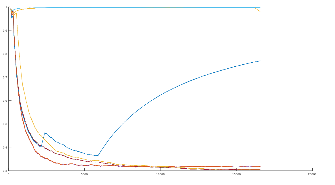
The average percentage of matching bases (y-axis) as a function of base index (x-axis).

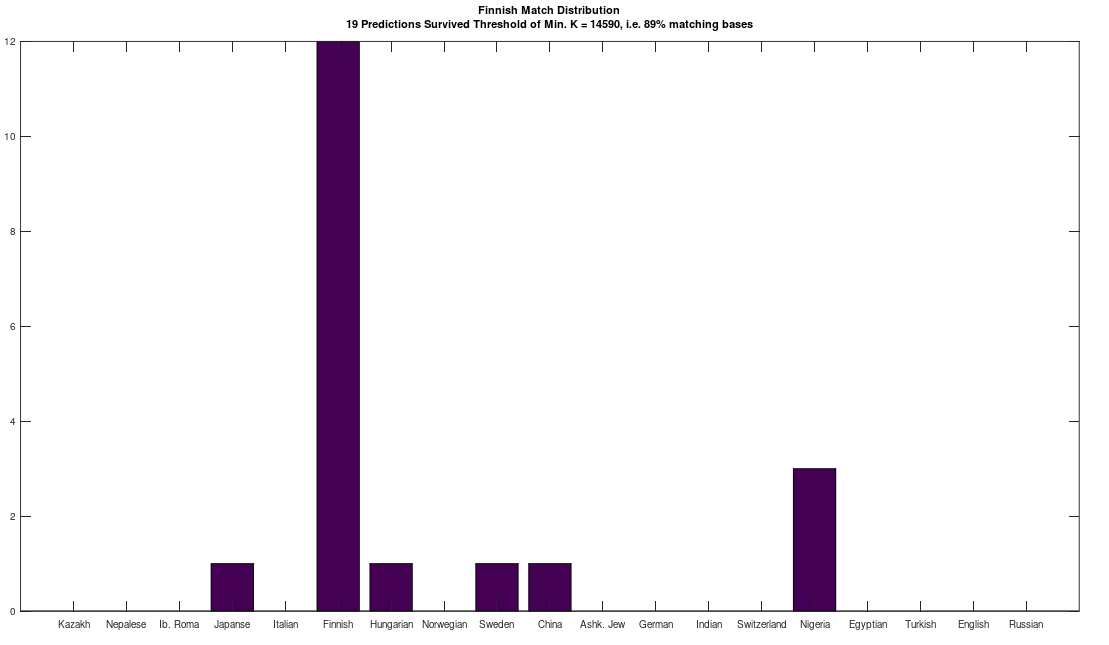
Specifically, if you count the average number of matching bases from index 1 to index K, using the NIH alignment, and increase K, you find that if two genomes in fact have a high number of matching bases, the curve plainly converges to around 99% to 100%. In contrast, two genomes that don’t match instead diverge from a high matching percentage to around 25% (i.e., chance). This produces curves that are useful for Machine Learning, since it implies an unsupervised clustering algorithm, where two genomes are clustered together if they produce an upward sloping curve, and are otherwise, not clustered together. Note that you don’t have to test the overall matching base percentage using this method, and it is therefore totally unsupervised.

The plot above shows 10 complete Nigerian mtDNA genomes compared to a single Japanese genome. The x-axis is the genome index, and the y-axis is the percentage of matching bases, from index 1 up to the x-value. Most of the Nigerian genomes plainly do not match, and so they diverge, whereas some plainly do (converging at the top). There’s also an outlier in the middle, which you can consider as a third class that is a partial match, or simply disregard, as the bottom line is, this produces a useful unsupervised clustering algorithm that could be used to group mtDNA genomes beyond obvious geographies or other known connections.

I’ve expanded this inquiry into four other species formally, and several others anecdotally, and it seems the same is true of those species. Moreover, differences in the otherwise common opening mtDNA sequences are plainly associated with significant morphological distinctions. For example, the Gorilla and Chimp genomes in the dataset have perfectly consistent opening sequences of length 193 and 19, respectively. In contrast, the Goat and Carp genomes have consistent opening sequences of length 1 and 2, respectively, though closer examination shows that subsets of those genome groups have substantial overlap in their opening sequences. One sensible interpretation, is that a long, consistent opening sequence is unique to Humans, Chimps, and Gorillas. Another interpretation is that Humans, Chimps, and Gorillas, are within their own species morphologically roughly homogenous, whereas the same is plainly not true of Carp and Goats, both of which contain a wide variety of what could be fairly described as subspecies or breeds. The images below shows plain morphological differences between the Black Bengal Goat, and the Jamnapari Goat, including different coloring, hair lengths, horn shape, and face shape.

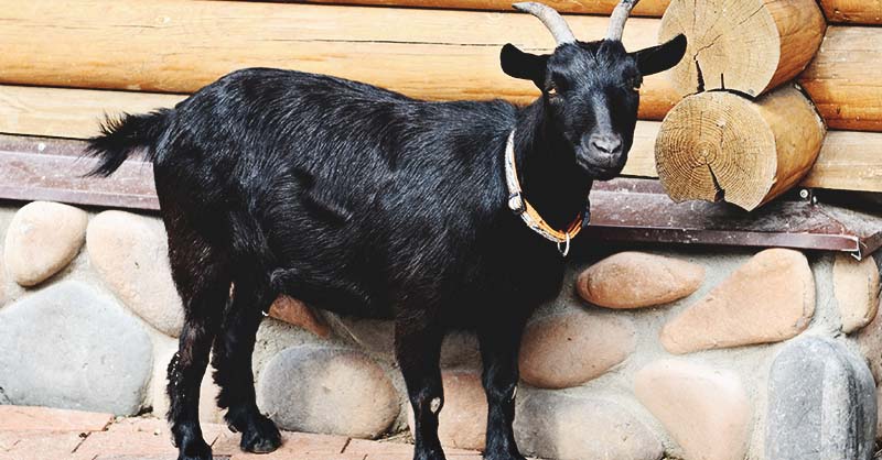
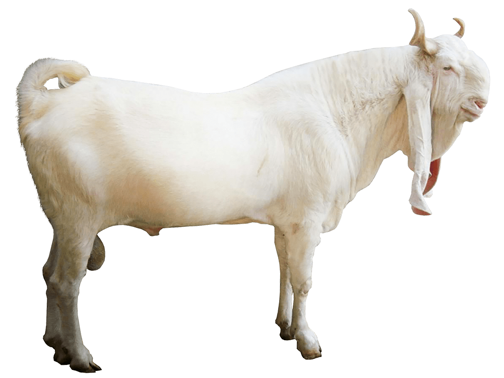
Bengal Black Goat (left) and a Jamnapari Goat (right).

It follows then that a morphologically consistent species such as the Emperor Penguin should produce alignments with a consistent opening sequence. Running a BLAST search for this specimen genome produces exactly that result, with a consistent opening sequence for the results returned. Simply look through the Alignment page, and you’ll note that there are no adjustments at all (i.e., the Subject index equals the Query index), and that the bases are consistent over the opening line of 60 bases. This is not a comprehensive study, but given that these are complete genomes, from a wide variety of human populations, and a reasonable number of non-human species, it is a credible hypothesis. Specifically, that variance in the opening sequence of an idealized alignment for a population of mtDNA genomes is consistent with significant morphological diversity. Further, it is also consistent with the hypothesis that the populations in scope should be subdivided until they produce a single opening sequence of appreciable length (i.e., beyond chance).

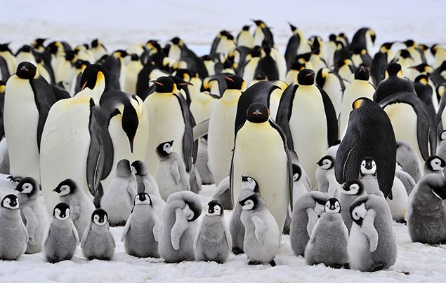
Emperor Penguins.

Note again that because mtDNA is circular, changes to the specific indexes are irrelevant, provided they are consistent, allowing us to compare what are then the opening sequences (i.e., shifting until we find the most consistent portion of the data across all genomes). In contrast, changes to the alignment that imply insertions or deletions are in fact significant. Moreover, in other contexts beyond mtDNA, insertions and deletions are plainly associated with morphological distinctions, specifically Down Syndrome and Williams Syndrome, as both produce distinct morphological changes to human beings, that are generally consistent in people with those disorders. Down Syndrome is due to a massive insertion, specifically an additional chromosome, and Williams Syndrome is due to specific deletions on Chromosome 7.

The net conclusion is that insertions and deletions in mtDNA seem to be associated with morphological variance, and because human beings are so superficially diverse, yet contain exactly the same opening sequence, it follows that the amount of variance required to generate significant differences in alignment should be quite drastic. There are however some examples within human populations that imply insertions and deletions, when compared to the majority of samples. Specifically, as I previously noted, some Japanese people have minor insertions and deletions to this opening sequence. More significantly, Iberian Roma are a near-perfect match with Homo Heidelbergensis (i.e., around 98% of bases matching), without any changes to the alignment of their mtDNA, using the standard NIH alignment. The code attached below will allow you to make this base-by-base comparison, without adjustment to alignment. In contrast, most other genomes in the dataset produce a number of matching bases around chance (i.e., around 28%) when compared to Heidelbergensis. This is astonishing, and running a BLAST search comparing e.g., an Italian genome to Heidelbergensis, the alignment is adjusted significantly, effectively deleting about 300 bases, producing again a match percentage of 97%. However, this completely ignores the observation that insertions and deletions are associated with drastic differences in morphologies, and behaviors. This at least suggests the possibility that populations that are close to Heidelbergensis, without adjusting alignment, have more in common in terms of appearance and behavior with Heidelbergensis, than those that don’t. At a minimum, it suggests that they have a closer genetic relationship to Heidelbergensis than the general population, that does not require adjustments to alignment to account for insertions and deletions unique to Heidelbergensis and some other apparently related populations. Note that both Iberian Roma and Heidelbergensis contain the exact same opening sequence above that is common to the vast majority of homo sapiens, suggesting that we are the same species, and simply variants of that species. The same is true of Denisovans and Neanderthals.

Below is some code that will allow you probe the dataset, together with the dataset itself, that now consists of 180 complete mtDNA human genomes from 18 geographic populations, 1 complete Heidelbergensis genome, and 20 complete non-human genomes from 4 different species, specifically, Gorilla, Chimpanzee, Goat, and Carp.

https://www.dropbox.com/s/i0ly3hlg0cvzet6/mtDNA_Prefix_CMDNLINE.m?dl=0

https://www.dropbox.com/s/br0krmjjkncms2t/Compare_to_H_Heidel_CMNDLINE.m?dl=0

https://www.dropbox.com/s/casfm3i07v0vefl/Count_Matching_Bases.m?dl=0

https://www.dropbox.com/s/lxq8gfb4h0p8edw/mtDNA.zip?dl=0

Posit a source that produces signals over time, and assume that you record the signals generated. If has a high entropy, then it is conceivable that the first several observations are all novel. To make this more concrete, assume draws from a uniform distribution over . The probability of producing two sequential observations is . The probability of producing two unequal observations is instead . As a consequence, it is more likely than not that the first two observations present two novel observations. Now assume instead that draws from the set , with the probability of at . This then implies that the probability of two novel observations is given by , whereas the probability of sequential ‘s or sequential ‘s is given by . As is evident, the higher the entropy of a distribution, the greater the likelihood of novelty, though I’ll concede this is not a formal proof.

This is interesting in and of itself, but there’s yet another consideration, which is that newness is associated with novelty anecdotally. However, we can now make this concrete, by treating novelty as a previously unobserved observation. This will produce an objective metric for novelty, which is given simply by the number of novel observations over time. That which is stable, is by definition unlikely to produce novelty. That which is volatile is by definition likely to produce novelty, with the entropy serving as a sensible measure of volatility. We have therefore yet another connection, which is to time. Specifically, in order for a source to have a low entropy, we must have a large number of observations. In contrast, a system can have a high entropy by simply having a large number of possibilities, for which we have e.g., only one observation for each. As a consequence, fixing our rate of observation, a system that has a low entropy must be old, in the literal sense, that we have a large number of observations, and therefore a significant historical record of its behavior. In contrast, a system that has maximal entropy requires only one observation of each state of the system, which by definition is the most likely outcome for any sequence of observations.

As a consequence, a low entropy system is consistent with a system that is old and stable. Note however, that a low entropy does not imply that it is old and stable, but is instead consistent with being old and stable. In contrast a high entropy system doesn’t really provide much information at all. And finally, this is consistent with my equation for Knowledge, given by , where I would be in this case the maximum entropy of a source, and is its entropy, leaving Knowledge as the balance between the two. Applied in this case, a low entropy system provides some knowledge about its history, whereas a high entropy system does not.

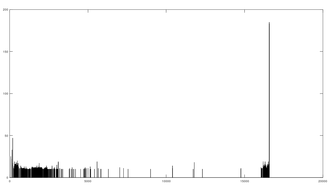
We can then consider the probability of novelty itself, disregarding the observed distribution of underlying outcomes. This allows us to consider the possibility of unforeseen events, and assign them a meaningful probability, as included in the category of novel events generally, which would in this view include unforeseen events.. This is something you cannot do generally with a fixed distribution. And again, we find that a low entropy distribution has a lower probability of producing novelty, when compared to a higher entropy distribution.

In a previous note, I pointed out that many (and possibly nearly all) human mtDNA genomes “begin” (i.e., despite its circularity) with exactly the same 15 bases:

GATCACAGGTCTATC

In fact, because it’s circular, it makes perfect sense that there is a starting index, otherwise you run the risk of beginning protein production at different indexes, given the same genome, thereby producing different proteins. Other species seem to have their own opening ledes as well. A very small number of genomes in the NIH database do not contain this lede, but this is extremely rare in what I’m assuming is an enormous database, and though I haven’t done any formal analysis, I’ve found only about a dozen entries that do not contain exactly this sequence in the opening of their ideal alignment, using BLAST. That is, about a dozen genomes still contain this sequence, but not in the opening of the alignment that maximizes the number of matching bases. Further, some Japanese genomes contain minor deletions from this opening sequence, and therefore require minor adjustments to this alignment. In contrast, some of the genomes I found using BLAST require significant adjustments, effectively deleting around 570 bases from the genome, suggesting a significant deviation from a typical human mtDNA genome.

This suggests that as a general matter the correct empirical alignment for the human mtDNA genome begins with this sequence, despite the fact that it is circular, suggesting a useful and arguably “correct” starting point index, and this is in fact reflected in the NIH database, with basically all human mtDNA genomes I’ve found aligned with this opening sequence (including the roughly 200 complete genomes assembled in the dataset below).

In that same note, I pointed out that if you use this alignment, which the NIH plainly does as a general matter, you find that matching genomes converge to a match, and genomes that don’t match, diverge. Specifically, if you count the average number of bases from index 1 to index K, and increase K, you find that two genomes that in fact have a high number of matching bases produce a curve that plainly converges to around 99% to 100%. In contrast, two genomes that don’t match instead diverge from a high matching percentage to around 25% (i.e., chance). This produces curves that are useful for Machine Learning, since it implies an unsupervised clustering algorithm, where two genomes are clustered together if they produce an upward sloping curve, and otherwise, not clustered together. The plot above shows 10 Nigerian mtDNA genomes compared to a single Japanese genome. The x-axis is the genome index, and the y-axis is the percentage of matching bases, from index 1 up to the x-value. Most of the Nigerian genomes plainly do not match, and so they diverge, whereas some plainly do (converging at the top). There’s also an outlier in the middle, which you can consider as a third class that is a partial match, or simply disregard, as the bottom line is, this produces a useful clustering algorithm.

As I tested this more, I realized that you can also build a distribution of the indexes of unequal bases. Specifically, for each genome, run Nearest Neighbor, and find the indexes where that genome and its Nearest Neighbor differ. This will create a distribution, where each index is associated with some number of genome pairs that disagree at that index. The higher that number, the greater the number of instances of unequal bases at that index. When you plot this, you find exactly the same distribution, where the number of anomalously high unequal bases tapers off, which is consistent with the curves plotted above, that produce convergence as a function of index. The bar chart above shows all peaks that exceed the average plus one standard deviation, though you can of course make use of variations on this. Note the peak at the end is due to the fact that basically all of the genomes are missing that entry, causing all of them to be treated as unequal at that index (i.e., the algorithm first calculates equal bases, and disregards all missing entries, causing the compliment to include all instances of missing entries). Considering this further, it implies regions that are common to genomes are found in between the peaks of the chart above. This should make it easy to find genes, and more generally, sequences common to populations, which presumably have some function, even if it’s simply indicative of genetic grouping.

Specifically, the code attached produces 984 roughly homogenous regions. We can then calculate the length of each such region. The total sequence length of the homogenous regions is 15,592 bases, and the total length of the genome is 16,576 bases. This leaves 984 bases unaccounted for, as highly variable regions. This is approximately the length of the D-Loop, also known as the non-coding region, which apparently is a “hot spot for mtDNA alterations“. As a general matter, mtDNA is dense with genes, suggesting that we shouldn’t have too many inconsistent regions, and in fact we don’t. Moreover, you can plainly see that the inconsistent regions become more sparse, with a highly inconsistent and contiguous region in the beginning that could very well be the D-loop.

This is therefore an unsupervised algorithm that apparently correctly partitions this genome.

Here’s the code and the dataset:

https://www.dropbox.com/s/0y881tw2s7w91c8/Temp_CMDNLINE_12_18.m?dl=0

https://www.dropbox.com/s/4m6fhz77ki2rtg8/Genetic_Nearest_Neighbor_Fast.m?dl=0

https://www.dropbox.com/s/4m6fhz77ki2rtg8/Genetic_Nearest_Neighbor_Fast.m?dl=0

https://www.dropbox.com/s/casfm3i07v0vefl/Count_Matching_Bases.m?dl=0

Dataset:

https://www.dropbox.com/s/ht5g2rqg090himo/mtDNA.zip?dl=0

There’s a plain structure to mtDNA, and astonishingly, every genome I’ve seen so far has exactly the same opening sequence of 15 characters, though some Asian peoples have deletions, but they’re otherwise exactly the same –

Literally the exact same opening sequence, globally, and it is as follows:

GATCACAGGTCTATC

This got me thinking that there’s an order to human mtDNA, that variation starts to take place after this opening, as a function of index. It seems that this is in fact the case. Even more interesting, when two genomes match beyond mere change, they produce a convergence towards the overall percentage of matching bases. That is, if you start at index 1, and read to the end of the genome, if two genomes match beyond chance, then the percentage of matching bases from 1 to the end starts to increase at a certain point. If instead, the two genomes have a match that is close to chance (i.e., roughly 1/4 of the bases match), then the percentage of matching bases decreases as a function of index. Here’s a plot of 10 Nigerian mtDNA genomes compared to a single Japanese genome. The x-axis is the genome index, and the y-axis is the percentage of matching bases, from index 1 up to the x-value.

This implies a clustering algorithm, where if the slope is negative on average, then it’s not a match. If instead the slope is positive on average, then there is a match.

Most of the Nigerian genomes are plainly not matches. However, there are two that are a 98% and 100% match to Japanese genomes, respectively (at the top). This implies unquestionable common maternal lineage. There’s a third, that you can see that seems to lag, and then catch up, which has a match percentage of 77%. This obviously implies a bit of judgment, but the algorithm makes perfect sense, and you can deal with these types of issues as you like.

The first and obvious takeaway is that political race is bull shit, and our history is questionable. The scientific takeaway is that mtDNA does seem to follow a chronology, from the first index to the last, and if this is true, then it seems there was an explosion of diversity in maternal lines early in our history, later leading to a convergence, more or less on par with modern maternal lines.

Here’s the code, anything missing (include datasets) can be found in the post just below this one:

https://www.dropbox.com/s/blzcyi7eyuqxu3a/Code%20%281%29.zip?dl=0

The Maritime Archaic mtDNA genomes available from the NIH Database are a 99% match (i.e., 99% of the bases match) for several European, African, and Asian people. Note these are complete genomes, and so it is impossible to deny common ancestry.

This is astonishing, because the strongest match is the Spanish, and this provides irrefutable evidence that people of European descent reached the Americas thousands of years before Columbus, as the Maritime Archaic people are dated somewhere between 7,500 and 3,500 years before present. You’ll also note that the Maritime Archaic samples are a 95% match to Homo Heidelbergensis, which is consistent with the hypothesis that Heidelbergensis is an ancestor common to all of humanity. Each chart shows the number of people in a given population that had a 99% match with the population in question. So the first chart shows the number of people from each population that had a 99% match to at least one Maritime Archaic genome. There are 10 rows in each population, over 17 populations, except for Heidelbergensis, for which only one complete genome is available.

The raw data together with the code and files providing provenance (i.e., direct links to the NIH Database for each row) are all available in two separate zip files:

https://www.dropbox.com/s/e0zf5eokcfdmi7s/MATLAB%20CODE.zip?dl=0

https://www.dropbox.com/s/lxq8gfb4h0p8edw/mtDNA.zip?dl=0

I suppose mtDNA doesn’t control much for superficial appearance, given these results, and the others I’ve been sharing lately, certainly not the factors we typically associate with race, but more remarkably, because it doesn’t change much over generations, it forces us to recognize the brevity of our considerations, that they’re informed by a few centuries or millennia, when the real history of humanity spans hundreds of thousands of years, possibly longer.

Using a simple measure of information, specifically , where is the size of a distribution, and is the entropy of the distribution, the Danes are the most diverse people in the world, with a 99% match to a simply astonishing variety of nationalities. Even more astonishing, if you lower the match threshold to about 95%, you’ll see that many modern populations are a match for Homo Heidelbergensis, an archaic human that was thought to have gone extinct hundreds of thousands of years ago, though it’s quite clear many modern humans are basically indistinguishable on their maternal line from this otherwise archaic species.

I suppose mtDNA doesn’t control much in the way of superficial appearance, given these results, and the others I’ve been sharing lately, certainly not the factors we typically associate with race, but more remarkably, because it doesn’t change much over generations, it forces us to recognize the brevity of our considerations, that they’re informed by a few centuries or millennia, when the real history of humanity spans hundreds of thousands of years, possibly longer. It’s not that this line of study doesn’t divide humanity, as it certainly does, but not along any political or racial basis I’ve seen before. Instead, more than anything else, it shows that our ideas of race are totally unscientific, and basically a myth.

I’ve updated the dataset to include the raw genomes and the provenance for each file, with a link to the NIH database entry for each row.

Enjoy!

https://www.dropbox.com/s/ht5g2rqg090himo/mtDNA.zip?dl=0

It turns out the Japanese do have unique mtDNA, but the alignment data provided by the NIH hides this, because it presents the first base of the genome as the first index, without any qualification, as there’s an obvious deletion to the opening sequence of bases. Maybe this is standard, but it’s certainly confusing, and completely wrecks small datasets, where you might not have another sequence with the same deletion. The NIH of course does, and that’s why BLAST returns perfect matches for genomes that contain deletions, and my software didn’t, because I only have 185 genomes.

The underlying paper that the genomes are related to is here:

https://pubmed.ncbi.nlm.nih.gov/34121089/

Again, there’s a blatant deletion in many Japanese mtDNA genomes, right in the opening sequence. This opening sequence is perfectly common to all other populations I sampled, meaning that the Japanese really do have a unique mtDNA genome.

Here’s the opening sequence that’s common globally, right in the opening 15 bases:

GATCACAGGTCTATC

For reference, here’s a Japanese genome with an obvious deletion in the first 15 bases, together for reference with an English genome:

https://www.ncbi.nlm.nih.gov/nuccore/LC597333.1?report=fasta

https://www.ncbi.nlm.nih.gov/nuccore/MK049278.1?report=fasta

Once you account for this by simply shifting the genome, you get perfectly reasonable match counts, around the total size of the mtDNA genome, just like every other population. That said, it’s unique to the Japanese, as far as I know, and that’s quite interesting, especially because they have great health outcomes as far as I’m aware, suggesting that the deletion doesn’t matter, despite being common to literally everyone else (as far as I can tell). Again, literally every other population (using 185 complete genomes) has a perfectly identical opening sequence that is 15 bases long, that is far too long to be the product of chance.

Here’s the updated software that finds the correct alignment accounting for the deletion:

https://www.dropbox.com/s/2lwgtjbzdariiik/Japanese_Delim_CMDNLINE.m?dl=0

I noticed that some Japanese people seem to have a very low number of bases in common with not only the world, but each other. The dataset I’m using consists of 185 complete genomes, from 19 nationalities, and 3 ancient species, all taken from the NIH Database.

For 2 of the 10 Japanese complete genomes, the maximum number of matching bases anywhere in the world is about 5,000 matching bases. The complete genome has a size of 16,579 bases, and so this is not much better than chance, given by 16,579/4 = 4.145, suggesting that it really is just the operation of chance causing any intersection at all between those Japanese genomes and the global population generally.

This view finds further support in the fact that the entire global population has a perfectly consistent genome (i.e., no variation at all) over the first 15 bases. The probability of this being chance is 1/4¹⁹⁰, which is so small, it’s zero in MATLAB. That is, the sequence has a length of 15, and it is common to 175 genomes.

Note this dataset includes 3 complete ancient genomes, specifically, Denisovan, Maritime Archaic, and Homo heidelbergensis, all of which also contain exactly the same globally common sequence. Homo heidelbergensis is thought to have gone extinct hundreds of thousands of years ago, suggesting there is basically zero variation in the opening prefix to human mtDNA.

Said otherwise, globally, there is no mutation at all over the first 15 bases of the human mtDNA genome, anywhere in known history.

This is not true when you include Japan, and in fact, only 1 genome out of 10 is a perfect match, and therefore consistent with the global genome. Instead, the average number of matches excluding that one individual, is 3.2, over the opening prefix of 15 bases.

Putting it all together, you have a global match count for 2 out of 10 Japanese people that seems to be the result of pure chance, and 9 out of 10 Japanese people have a prefix segment that is almost entirely inconsistent with a globally and historically uniform segment of mtDNA.

Has anyone noticed this before or heard other people discussing it? I think it’s consistent with one of two hypotheses:

1. Japanese mtDNA has a much higher rate of mutation than typical mtDNA, for whatever reason. We could test for this by looking at the rate of change from one generation to the next.
2. Japanese mtDNA descends from a totally different bacteria.
3. There was an event that caused a drastic mutation to Japanese mtDNA, and then natural selection took over, and so nothing much changed, since as far as I know, the Japanese have no drastically higher rates of diseases connected to mtDNA, and in fact they have good health outcomes overall.

If either 1 or 3 are true, then it suggests that DNA could have an error correcting function, since single base variants often produce disease, yet here we have drastically inconsistent mtDNA, that doesn’t seem to have any notable problems at all. Note that natural selection would certainly kill off bad outcomes, but it doesn’t produce good outcomes. And so this particular case is at least consistent with the idea that DNA can adjust mutated sequences to avoid malfunction and disease.

In any case, this is highly unusual, since mtDNA is consistent for generations, and in some cases over possibly hundreds of thousands of years. I’ll add the caveat that it could be bad data, despite being from a reputable source, and the opening prefix being inconsistent is perhaps evidence of this.

Here’s the dataset with a ton of code you can use to analyze the data, and here’s the search string for the raw data from the NIH Database.

I’m still tweaking this, but this is an algorithm for finding common ancestry given mtDNA (it will not work otherwise), and the best fit for a common ancestor to a population.

https://www.dropbox.com/s/yxvqgt73gfxxqlo/Root_Testing_CMNDLINE.m?dl=0

I’ve never been able to prove formally why my unsupervised classification algorithm works, and in fact, I’ve only been able to provide a loose intuition, rooted in how I discovered it: as you tighten the focus of a camera lens, the changes near the correct focus are non-linear, in that the object quickly comes into focus. And so I searched for the greatest change in the structure of a dataset as a function of discernment, which works incredibly well, especially for an unsupervised algorithm. In contrast, the supervised version of that algorithm has a simple proof, which you can find in my paper Analyzing Dataset Consistency. However, it just dawned on me, I think I explained why it works, though it’s not a formal proof, in my other paper, Information, Knowledge and Uncertainty. Specifically, the opening example I give is a set of boxes, one of which contains a pebble, where the task is to guess which box the pebble is in. If someone tells you that the pebble is not in the i-th box, then your uncertainty is reduced. But the reason it’s reduced is because the system is now equivalent to a system with one less box. In contrast, the rest of the examples I give in that paper, deal with static observations that have some fixed uncertainty.

Applying this to my unsupervised clustering algorithm, the point at which the entropy changes the most (i.e., Uncertainty), is also the point at which your Knowledge changes the most, due to the simple equation . As a consequence, my unsupervised clustering algorithm finds the point at which your knowledge changes the most as a function of the structure of the dataset. All points past that, reduce the size, and therefore information content of the clusters, without materially adding to Knowledge. Specifically, if you unpack the equation a bit more, , where is the number of states of the system. In the case of the box example, is the number of boxes when there’s one pebble. In the case of a distribution, it’s the total number of elements in the distribution. And as you’re increasing the threshold for inclusion in a cluster, the cluster size shrinks, thereby decreasing . If it turns out that the size of the problem space generally decreases faster than the entropy (i.e., Uncertainty U), then your Knowledge actually decreases as the problem space decreases in size. As a consequence, the unsupervised algorithm finds the point where the entropy of the problem space changes the most as a function of the threshold for inclusion, which is the point where you get the most Knowledge per unit of change. I suppose upon reflection, the correct method is to find the point where the entropy of the problem space changes the most as a function of the size of the problem space. That said, my software plainly works, so there’s that.

In any case, this is not a proof, but it is a mathematical explanation. What I’m starting to come around to, is the idea that some phenomena, perhaps even some algorithms, function as a consequence of epistemological truths of reality itself. You can definitely accuse me of laziness, in that I can’t formally prove why the algorithm works, but that dismisses the possibility that some things might be true from first principles that defy any further logical justification, in that they form axioms consistent with reality itself. In that case, there is no proof beyond the empirical fact that Knowledge changes sub-optimally past the point identified by the algorithm. The reason I believe this is possible, is because the equation , follows solely from the tautology that all things are either in a set, or not, and there is, as far as I know, no other proof that this is true. Moreover, the equation works, empirically, so it is in this view an equation that has no further logical justification, that operates like an equation of physics. The more general premise at least suggests the possibility of algorithms that defy further logical justification beyond empiricism.

The reason I thought of this, is because I was working on clustering populations on the basis of mtDNA, and I noticed the same thing happen that happened when I first started my work in A.I. –

There was a massive discontinuous change in cluster entropy, as a function of the inclusion threshold. When I looked at the results, it produced meaningful population clusters, where e.g., both Japanese and Finnish people are treated as homogenous, and basically everyone else is heterogenous. This was totally unsupervised, with no information at all, other than raw mtDNA, and it’s obviously correct. Moreover, Sweden and Norway produced basically the same heritage profile, and even terminate at exactly the same iterator value –

This is consistent with the fact that Norwegians and Swedes are genetically closer to each other than they are to the Finns. The Finns also speak a totally different, Uralic language, whereas Norwegian and Swedish are both Germanic, and so in this case, heritage follows language, which is not necessarily always true, for the simple reason of conquest. For example, the Swedes and Norwegians had their own alphabet, the Runic Scripts, and now they don’t, they use the Latin alphabet like everyone else, because of what is basically conquest.

Above are the plots for the Finnish, Japanese, Swedish, and Norwegian heritage profiles I mentioned, and below is the code and a link to the dataset. You might be wondering how it is that of the few populations that map to Finland, Nigeria is among them. Well, it turns out, 87% of the complete Finnish mtDNA genome maps to a 2,000 year old Ancient Egyptian genome. They also map basically just as closely to modern Egyptians. All of this data is from the National Institute of Health, and you can find all of it by entering the following search query into the NIH Database:

ETHNICITY AND ddbj_embl_genbank[filter] AND txid9606[orgn:noexp] AND complete-genome[title] AND mitochondrion[filter]

Just replace ETHNICITY with Norway, Egypt, etc. Isn’t life something when you actually do the work.

Here’s the code:

https://www.dropbox.com/s/h8ae0tuvtoa1bk1/Percentage_Based_Clustering_CMDNLINE.m?dl=0

Here’s the dataset:

https://www.dropbox.com/s/mj8qk8jxybc9wbc/MTDNA.txt?dl=0

The dataset now includes 19 ethnicities (listed below), and it’s simply fascinating to dig into, and there’s a bunch of software in the previous posts you can use to probe it.

Kazakh, Nepalese, Iberian Roma, Japanese, Italian, Finnish, Hungarian, Norwegian, Sweden, Chinese, Ashkenazi Jewish, German, Indian, Switzerland, Nigerian, Egyptian, Turkish, English, Russian.