I realized the other day that the equations I present in Section 3.3 of my paper, A Computational Model of Time-Dilation, might imply that wave behavior will occur with a single particle. I need to go through the math, but the basic idea is that each quantized chunk of mass energy in an elementary particle is actually independent, and has its own kinetic energy. This would allow a single elementary particle to effectively sublimate, behaving like a wave. The point of the section is that on average, it should still behave like a single particle, but I completely ignored the possibility that it doesn’t, at least at times, because I wanted single particle behavior, for other sections of the paper. I was reminded of this, because I saw an experiment, where a single neutron plainly travels two independent paths. If the math works out, we could completely ditch superposition, since there’s no magic to it, the particle actually moves like a wave, but generally behaves like a single particle. That said, I think we’re stuck with entanglement, which seams real, and I still don’t understand how it works, but nothing about entanglement contradicts my model of physics.
Author: erdosfan
Note on Ramsey’s Theorem
It’s always bothered me that Ramsey’s Theorem is not probabilistic. For example, R(3,3), i.e., the smallest order complete graph that contains either a complete graph on 3 vertices, or an empty graph on 3 vertices, is 6. This means that literally every graph with 6 or more vertices contains either a complete graph on e vertices, or an empty graph on e vertices. This is not probabilistic, because it’s simply true, for all graphs on 6 or more vertices. But it just dawned on me, you can construct a probabilistic view of this fact, which is that on fewer than 6 vertices, the probability is less than one, whereas with 6 or more vertices, the probability is 1. This is true in the literal sense, since less than all graphs with fewer than 6 vertices have a complete graph on 3 vertices, or an empty graph on 3 vertices, but some will. I think this could actually be quite deep, and connect to random graphs, but I need some time to think about it.
Another thought, that I think I’ve expressed before, if we can analogize Ramsey’s Theorem to time, then it would imply that certain structures eventually become permanent. This is a truly strange idea, and though I’m just brain storming, intuitively, it doesn’t sound wrong. And now that I’ve thought a bit more about it, I’ve definitely had this idea before:
Specifically, correlation between two random variables can be thought of as an edge between two vertices, where the vertices represent the variables, and the edge represents the presence or absence of correlation. If we consider all random variables together, then it’s clear that having no correlation at all would correspond to an empty graph, and correlation between all variables would correspond to a complete graph. If all graphs are equally likely, no correlation, and total correlation would be equally likely, and in fact the least likely possibilities for any graph with more than two vertices (when compared to at least some but less than total correlation). As a result, if we randomly select, random variables, we should generally find at least some correlation, regardless of their nature or apparent relationships.
If we imagine time quantized on a line, with a vertex representing a moment, and allow for one moment in time to be related to another moment in time by connecting them with an edge, we will have a graph, that just happens to be visualized along a line. Applying Ramsey Theory, we know that certain structures must emerge over time, since we are allowing for the possibility of ever larger graphs. At the same time, the correlation argument above implies that each moment should have some possibly non-causal connection to other moments, producing non-empty graphs. That is, if one moment is connected to another in the remote past, it’s really not credible that it’s causal, and is instead an artifact of this line of thinking. This argument as a whole implies the possibility that reality has non-causal relationships over time, regardless of whether or not the past, present, or future, is memorialized in any way, and regardless of whether or not the past, present, or future is physically real, because these are immutable, abstract, arguments. All of that said, this is a lot to think about, and I need to organize it a bit more, but the core idea seems sound, and that’s disturbing.
Reconsidering the Origins of Humanity
I first thought that the Denisovans were the original maternal line for humanity, i.e., the common ancestor of all modern humans. I do not think that’s the case any longer, and instead, it seems it’s literally the Romani people, who are in turn the ancestors of Heidelbergensis. Heidelbergensis seems to be the ancestor of the Phoenicians, and the Phoenicians are in turn the ancestors of the Old Kingdom Egyptians. The Old Kingdom Egyptian maternal line is literally everywhere in the world, Europe, Africa, Asia, and seems to be the defining maternal line of modern people. This is the result of more careful application of my ancestry algorithm that I describe here.
What’s strange (frankly) about the Romani people, is that they seem to have a single maternal ancestor. That is, if you apply clustering to the Romani maternal line, you find exactly one cluster, suggesting all of the maternal lines in the Romani people are basically identical. This is not a small dataset, but it’s not every living person, so it’s possible that there’s more than one. However, the bottom line is, humanity would in this hypothesis descend from either an individual maternal ancestor, or a single family.
Ordinal Ranking of Complexity Across UTMs
I’m still working on this, but it looks like if K(x) < K(y), on a given UTM, where K(x) denotes the Kolmogorov complexity of the string x, there’s no guarantee, absent additional assumptions, that K(x) < K(y) on some other UTM. This is a big deal if true, because the difference in the Kolmogorov Complexities across two UTMs is always bounded by a constant, suggesting universality. But if the ordinal ranking of complexities is not generally preserved across UTMs, then we can’t say it’s truly universal. It looks like the answer is that for sufficiently different strings where |K(x) – K(y)| is large, then order is preserved, but still, this is a big deal that I’ve never seen mentioned anywhere. I’ll follow up shortly with a proof if it’s actually correct.
UPDATE: Here’s the proof so far.
Complexity on Different UTMs: Many machines are mathematically equivalent to a UTM, and as a consequence, there are multiple UTMs. For example, Charles Babbage’s Analytical Engine is a UTM, and so are basically all personal computers.
However, there’s a simple lemma that proves the difference between K(x) for any two UTMs is bounded by a constant C that does not depend upon x.
Example: Let’s assume that both Octave and Python are “Turing Complete”, which means you can calculate any function, or more generally run any program, that you can run on a UTM in both Octave and Python. Anything you can run on a UTM is called a “computable function”.
This means (arguendo) that any computable function can be implemented in both Octave and Python, which is probably true.
The compilers for both Octave and Python are themselves computable functions. This means that we can write a Python compiler in Octave, and vice versa. As a consequence, given a program written in Python, we can compile that program in Octave, using a single, universal compiler for Python code that runs in Octave. This code will have a fixed length C.
Let KO(x) and KP(x) denote length of the shortest program that generates x as output in Octave and Python, respectively, and assume that y is the shortest Python program that generates x, so that KP(x) = |y|.
Because we have a compiler for Python code that runs in Octave, we can generate x given y and that compiler, which together will have a length of,
KP(x) + C ≤ KO(x).
Said in words, the complexity of x in Octave can’t be greater than the complexity of the Python program that generates x, plus the Python compiler that runs in Octave, for all x.
Further, this argument would apply to any pair of Turing Complete languages, which implies the following general result:
K1(x) + C ≤ K2(x), Eq. (1)
where C is a constant that does not depend upon x, and K1(x) and K2(x) are the Kolmogorov Complexities of x in two distinct Turing Complete languages.
Consistency of Ordinality: Ideally, the ordinal rankings of strings in terms of their complexities would be consistent across UTMs, so that if K1(x) < K1(y), then K2(x) < K2(y). If true, this would allow us to say that x is less complex than y, on an objective basis, across all UTMs.
This is the case, subject to a qualification:
Assume that K1(x) < K1(y). Eq. (1) implies that,
K1(x) ≤ K2(x) + C; and
K1(y) ≤ K2(y) + C, for exactly the same value of C.
This in turn implies that,
K1(x) = K2(x) + c_x; and
K1(y) = K2(y) + c_y, for some c_x, c_y ≤ C.
That is, Eq. (1) implies that there must be some exact values for c_x and c_y that are both bounded above by C, and possibly negative.
We have then that,
K2(x) = K1(x) – c_x; and
K2(y) = K1(y) – c_y.
Because we assumed K1(x) < K1(y), if c_y ≤ c_x, then the result is proven. So assume instead that c_x ≤ c_y. Now set,
c_x = K1(x) – K1(y) + c_y, which implies that
K2(x) = K1(x) – K1(x) + K1(y) – c_y = K2(y).
As a consequence, for any c, such that c_x < c ≤ C, it must be the case that K1(x) – c = K2(x) < K2(y), which is exactly the desired result. Simplifying, we have the following constraint, satisfaction of which will guarantee that K2(x) < K2(y), noting that |c_y – c_x| < C:
C < K1(y) – K1(x). Eq. (2)
Said in words, if we know that the difference in complexities between strings x and y, exceeds the complexity of the translator compiler between the machines, then their ordinal relationships are preserved. However, this means that ordinality could be sensitive to differences in complexity that are small relative to the compiler.
UPDATE 2:
It just dawned on me, the Halting Problem is a physical problem, that cannot be answered, because of decidability, not because of some mechanical limitation. That is, there is a logical contradiction, which precludes existence. Because UTMs are physically real, we have a mathematical result that proves the non-existence of some physical system, specifically, a machine that can solve the Halting Problem.
Determining Order without Entropy
I’m working on another ancestry algorithm, and the premise is really simple: you simply run nearest neighbor on every genome in a dataset. The nearest neighbors will produce a graph, with every genome connected to its nearest neighbor by an edge. Because reality seems to be continuous as a function of a time, small changes in time, should produce small changes in genomes. Because nearest neighbor finds you the smallest difference between a given genome and another over a given dataset, it follows that if genome A is the nearest neighbor of B, then A and B are most proximate in time, at least limited to the dataset in question. However, it’s not clear whether A runs to B, or B runs to A. And this is true, even given a sequence of nearest neighbors, ABC, which could be read either forwards or backwards. That is, all we know is that the genomes A, B, and C are nearest neighbors in that order (i.e., B is the nearest neighbor of A, and C is the nearest neighbor of B).
This is something I came up with a long time ago, using images. Specifically, if you take a set of images from a movie, and remove the order information, you can still construct realistic looking sequences by just using nearest neighbor as described above. This is because reality is continuous, and so images that are played in sequence, where frame i is very similar to frame i + 1, creates convincing looking video, even if it’s the wrong order, or the sequence never really happened at all. I’m pretty sure this is what the supposedly “generative A.I.” algorithms do, and, frankly, I think they stole it from me, since this idea is years old at this point.
However, observing a set of images running backwards will eventually start to look weird, because people will walk backwards, smoke will move the wrong direction, etc., providing visual cues that what you’re looking at isn’t real. This intuitive check is not there with genomes, and so, it’s not obvious how to determine whether the graph generated using nearest neighbor is forwards or backwards in time.
This lead me to an interesting observation, which is that, there’s an abstract principle at work, that the present should have increasingly less in common with the future. Unfortunately, this is true backwards or forwards, but it does add an additional test, that allows us to say, whether or not a sequence of genomes is in some sensible, temporal order. Specifically, using ABC again, A and B, should have more bases in common, than A and C, and this should continue down the sequence. That is, if we had a longer sequence of N genomes, then genome 1 should have less and less in common with genome i, as i increases.
For datasets generally, we still can’t say whether the sequence is backwards or forwards, but we can say whether the sequence is a realistic temporal embedding, and if so, we will know that it yields useful information about order. However, because mutation is random, in the specific case of genomes, if it turns out that A and B contain more bases in common than A and C, then that can’t realistically be read backwards from C to A, which would imply that C randomly mutated to have more bases in common with A, which is not realistic for any appreciable number of bases. This is analogous to smoke running backwards, which just doesn’t happen. However, because of natural selection, we can’t be confident that entropy is increasing from A to C. In fact, if genomes became noisier over time, everyone would probably die. Instead, life gets larger, and more complex, suggesting entropy is actually decreasing. That said, we know that the laws of probability imply that the number of matching bases must decrease between A and all other genomes down the chain, if A is in fact the ancestor of all genomes in the chain. But this is distinct from entropy increasing from A onwards. So the general point remains, you can determine order, without entropy.
UPDATE: It just dawned on me, that if you have a particle that has uniform, random motion, then it’s expected change in position is zero. As a result, if you repeatedly observe that particle moving from a single origin point (i.e., its motion always commences from the same origin), its net motion over time will be roughly zero, but you’ll still have some motion in general. If a given point constantly ends up a terminus in the nearest neighbor construction above, then it’s probably the origin. The reasoning here is that it’s basically impossible for the same point to appear as a terminus, unless it’s the origin. I think this implies that a high in-degree in the nearest neighbor graph over genomes above, implies that genome is a common ancestor, and not a descendant.
Collection of Posts
I’ve assembled basically all of the posts on this blog into a single zip file of pdfs, which you can download here.
Enjoy!
Charles
Spatial Uncertainty and Order
I presented a measure of spatial uncertainty in my paper, Sorting, Information, and Recursion [1], specifically, equation (1). I proved a theorem in [1] that equation (1) is maximized when all of its arguments are equal. See, Theorem 3.2 of [1]. This is really interesting, because the same is true of the Shannon Entropy, which is maximized when all probabilities are equal. They are not the same equation, but they’re similar, and both are rooted in the logarithm. However, my equation takes real number lengths or vectors as inputs, whereas Shannon’s equations takes probabilities as inputs.
I just realized, that Theorem 3.2 in [1], implies the astonishing result, that the order of a set of observations, impacts the uncertainty associated with those observations. That is, we’re used to taking a set of observations, and ignoring the ordinal aspect of the data, unless it’s explicitly a time series. Instead, Theorem 3.2 implies that the order in which the data was generated is always relevant in terms of the uncertainty associated with the data.
This sounds crazy, but I’ve already shown empirically, that these types of results in information theory work out in the real world. See, Information, Knowledge, and Uncertainty [2]. The results in [2], allow us to take a set of classification predictions, and assign a confidence value to them, that are empirically correct, in the sense that accuracy increases as a function of confidence. The extension here, is that spatial uncertainty is also governed by an entropy-type equation, specially equation (1), which is order dependent. We could test this empirically, by simply measuring whether or not prediction error, is actually impacted by order, in an amount greater than chance. That is, we filter predictions, as a function of spatial uncertainty, and test whether or not prediction accuracy improves as we decrease uncertainty.
Perhaps most interesting, because equation (1) is order dependent, if we have an observed uncertainty for a dataset (e.g., implied from prediction error), and we for whatever reason do not know the order in which the observations were made, we can then set equation (1) equal to that observed uncertainty, and solve for potential orderings that produce values approximately equal to that observed uncertainty. This would allow us to take a set of observations, for which the order is unknown, and limit the space of possible orderings, given a known uncertainty, which can again be implied from known error. This could allow for implications regarding order that exceed a given sample rate. That is, if our sample rate is slower than the movement of the system we’re observing, we might be able to restrict the set of possible states of the system using equation (1), thereby effectively improving our sample rate in that regard. Said otherwise, equation (1) could allow us to know about the behavior of a system between the moments we’re able to observe it. Given that humanity already has sensors and cameras with very high sample rates, this could push things even further, giving us visibility into previously inaccessible fractions of time, perhaps illuminating the fundamental unit of time.
The Rate of Mutation of mtDNA
I’ve written in the past on the topic of the rate of mutation of mtDNA, in an attempt to calculate the age of mankind. It turns out, there really isn’t a good single answer to the rate at which human mtDNA mutates, and as a result, you really can’t come to any clear answer using mtDNA alone. And in fact, I realized the other day, that it seems to vary by maternal line. Specifically, some modern humans carry archaic mtDNA, in particular Heidelbergensis, Denisovan, and Neanderthal mtDNA. Other modern humans carry mtDNA that is basically identical to ancient mtDNA (e.g., 4,000 years old), but not archaic mtDNA (e.g., 100,000 years old). In particular, many modern humans globally carry Ancient Egyptian mtDNA, from about 4,000 years ago.
You can get an idea of the rate of mutation, by taking e.g., a modern human that has Denisovan mtDNA, and comparing that to a bona fide archaic Denisovan genome, count the number of changed bases, and then divide by the number of years since the archaic sample lived, which will produce a measure of the number of changed bases per year. This can of course be expressed as a percentage of the total genome size, which is what I’ve done below.
We can be a bit fancier about it, by comparing a given genome to many others, producing a distribution of the number of changed bases per year. The code below does exactly this, producing the average total percentage change, minimum total change, maximum total change, and standard deviation over all total changes. The comparison was made only to modern genomes, and so we can take the known (and plainly approximate) date of the archaic / ancient genome, and divide by the number of years to the present. This will produce a rate of change per year, which I’ve expressed as a rate of change per 1,000 years.
The results are as follows:
| Genome Type | Avg. Change | Min. Change | Max. Change | Std. Deviation | Genome Date | Avg. Change Per 1000 Years |
| Denisovan | 26.39% | 25.76% | 32.70% | 1.99% | 120,000 BP | 0.22% |
| Neanderthal | 3.74% | 2.79% | 36.60% | 3.27% | 80,000 BP | 0.047% |
| Heidelbergensis | 4.27% | 3.30% | 37.61% | 3.30% | 430,000 BP | 0.0099% |
| Ancient Egyptian | 3.74% | 0.17% | 35.23% | 8.32% | 4,000 BP | .935% |
Again, note that Denisovan, Neanderthal, and Heidelbergensis are all archaic humans. In contrast, the Ancient Egyptians are of course ancient, but not archaic. The dataset contains 664 rows, 76 of which are archaic or ancient, which leaves 588 rows for the comparisons produced above. As a result, even though the table above was produced using only 4 input genomes, the results were generated comparing each of the 4 input genomes to all 588 complete, modern human mtDNA genomes in the dataset. The plain implication is that modern human mtDNA is evolving faster than archaic human mtDNA, since, e.g., the Ancient Egyptian genome has an average total rate of change equal to that of the Neanderthals, despite having only 4,000 years to achieve this total change, in contrast to the roughly 120,000 years that have passed since the Neanderthal genome. Technically, we should only be testing genomes we believe to be descended from the archaic / ancient genomes, since e.g., it is theoretically possible that a modern person has mtDNA that predates the Ancient Egyptian genome, since mtDNA is so stable. That said, the bottom line is that this is a measure of the variability of a particular maternal line, and the amount of mutation cannot exceed that variability. For this and other reasons, more studies are required, but this is an interesting observation.
The code is below, the balance of the code can be found in my paper, A New Model of Computational Genomics.
Update on Norwegian Ancestry
I wrote a note a while back on Norwegian ancestry [1], and in that note I show that about 14% of Norwegians have Thai mtDNA, whereas about 6% of Swedes have Thai mtDNA. The match threshold is in this case set to 99% of the full mtDNA genome, so this is not something that can be dismissed. Further, the Finns are even closer to the Thai, with about 18% of Finns again a 99% match to Thai mtDNA. Sweden is in the middle of Norway and Finland, so it’s a bit strange, since you can’t argue an East to West migration, unless the Swedes killed a lot of people that are related to the Thai, or simply didn’t reproduce with them.
I think instead we can make sense of all of this, by looking to the Sami, who are yet again even closer to the Thai, with about 30% of the Sami a 99% match to the Thai. The Sami are nomadic people that certainly extend further East than the Scandinavians, into Russia, and I think they are ultimately Asian people. If true, this would explain why the Finns are so close to the Thai, and then all you need is for the Swedes to generally avoid mating with the Finns, which is what sovereign boundaries generally accomplish. The fact that the Finns and Sami speak a totally different, Uralic language, whereas the Swedes and Norwegians speak Germanic languages, is consistent with this hypothesis.
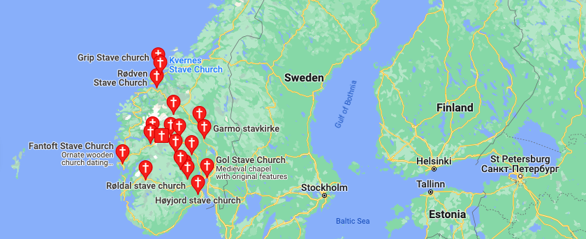
This still leaves the question of why the Norwegians are so close to the Thai. I previously noted in [1] that Norway, and not Sweden, has a large number of churches, that are plainly Asian in design, and Thai in particular. Below is (1 left) the distribution of Stave Churches, none of which are in Sweden, though they are elsewhere in Europe, (2 center) the Borgund Stave Church, and (3 right) the Sanctuary of Truth in Thailand.
The question is, why were these churches (all built around 800 years ago) only built in Norway, and not Sweden, and further, how on Earth did Thai mtDNA end up in Norway in such a large quantity?


I think the answer is actually quite simple: Nordic people travelled to Thailand, which is consistent with the fact that the Vikings had Buddhist relics. Further, I can’t find a single Viking monument that is still standing, other than the Runic Stones, basically all of which are in Sweden. I think Nordic people, presumably the Vikings, travelled to what is now Thailand, and learned how to construct buildings that last, out of wood. This might sound backwards from the basically racist modern perspective, but the Khmer Empire e.g., constructed massive temples that are still standing to this day, and had very advanced skills in the fine arts generally. Below is (1 left) Angkor Wat and (2 right) is a bust of Jayavarman VII, both of which are plainly superior in quality to anything produced by the Vikings, by a simply enormous margin, except the Viking ships. Both of these were again produced about 800 years ago, the same age as the Stave Churches.


Despite having drastically superior building and artisan skills generally, it seems at least credible that the people of South East Asia, around the time of the Khmer Empire, didn’t have the best ships. That AP article says that the Khmer Empire ship in question was cut from a single tree trunk. That is nothing compared to the ships constructed by the Vikings, which were at their extremes, almost three times as large, and extremely complex structures. Below is (1 left) the Oseburg ship, built around 1,200 years ago, (2 right) a detail from the Oseburg ship, and (3 right) a detail from the Urnes Stave Church, which is plainly similar to the detail from the Oseburg ship (and neither look terribly Christian to me).


Again, the Khmer ship is from almost exactly the time these Stave Churches are believed to have been built, about 800 years ago. This suggests the possibility that a bargain was struck, where a people that knew how to construct large, durable buildings (i.e., the South East Asians), exchanged that knowledge, for the ability to build large durable ships, or simply bought them from the Nordic people. A really interesting possibility is that this led to the settlement of Hawaii, which would obviously require seriously advanced navigation skills. Hawaii was believed to be settled around the same time, roughly 800 years ago, but this is still not totally sorted (to my limited knowledge on the topic). If you look through my work on mtDNA generally, you’ll see that about 50% of the Thai are a 99% match to the Hawaiians, making this a not totally ridiculous hypothesis.
The bottom line is, the Vikings probably didn’t know how to construct large durable buildings, until either someone figured it out, or someone else taught them. At the same time, if this is true, they sailed all the way to South East Asia, which is an astonishing accomplishment. In the case of the Khmer, it seems plausible that what was plainly an incredibly advanced civilization, was still making use of primitive boats.
All of this cuts again the false notion of generalized skill, and advancement, that probably comes from the Renaissance, and was reinforced in modernity, where one country is simply “more advanced” than another. In contrast, it seems plausible that people traded in ideas, a very long time ago, becoming skilled at only particular things, and learning other skills over time from other civilizations, creating a much more complex portrait of what I suppose would be a balance of trade. This would be an early market for intellectual property, that of course makes sense, it’s just not typically expressed in these terms, because it’s history and not economics, but in this view, history is economics.
All that said, the Thai are not the Khmer, but it’s pretty close. Further, the fact that the Nordic peoples went from building (as far as I can find) literally nothing that is still standing, to building plainly Asian structures that are still standing, suggests some kind of technology transfer. My best guess is that in exchange for knowledge, or perhaps simply ships, the Nordic peoples learned about real architecture from people that lived around what is now Thailand and Cambodia, and kept the style. Now, if you did all of this, you probably wouldn’t want to share any of it, especially if you brought back women, men being who they are, in particular Viking men. This would make it perfectly sensible to seek a separate piece of land, and start what I think was a distinct Nordic culture, that eventually came to be what we know as Norway.
Knowledge and Utility
I wrote a paper a while back called “Information, Knowledge, and Uncertainty” [1], that presents a mathematical theory of epistemology. I go on to apply it, showing that it can be used in machine learning to drastically improve the accuracy of predictions, using a measure of confidence that follows from the definitions in [1]. In some other research note that I don’t remember the name of, I pointed out that we can also think about a different kind of information that is conveyed through a proof. Specifically, that longer proofs correspond to more computational work, i.e., the work required to prove the theorem, which will have some number of deductive steps. Simply count the steps, the more steps there are, the more work required to prove the result. Now of course, you could have a “bad” and pointlessly long proof for a theorem. Simply posit the existence of a shortest proof, as an analog to the Kolmogorov Complexity. The number of steps in the shortest proof for a theorem is the depth of the theorem.
What caught my attention this morning is the potential connection between utility and the depth of a theorem. For example, the Pythagorean Theorem has very short proofs, and as a result, the shortest proof will necessarily also be short. Despite this, the Pythagorean Theorem is remarkably useful, and has undoubtedly been used relentlessly in architecture, art, and probably plenty of other areas of application. Now you could argue that there is no connection between depth and utility, but perhaps there is. And the reason I think there might be, is because I show that in [1], the more Knowledge you have in a dataset, the more accurate the predictions are, implying utility is a function of Knowledge, which has units of bits.
You can view the number of steps in a proof as computational work, which has units of changes in bits, which is different than bits, but plainly a form information. So the question becomes, is this something universal, in that when information is appropriately measured, that utility becomes a function of information? If this is true, then results like the Graph Minor Theorem and the Four Color Theorem could have profound utility, since these theorems are monstrously deep results. If you’re a cartographer or someone that designs flags, then the Four Color Theorem is already useful, but jokes aside, the point is, at least the potential, for profound utilization of what are currently only theoretical results.
As a self-congratulatory example, I proved a mathematical equivalence between sorting a list of real numbers and the Nearest Neighbor method [2]. The proof is about one page, and I don’t think you can get much shorter than what’s there. But, the point is, in the context of this note, that the utility is unreal, in that machine learning is reduced to sorting a list of numbers (there’s another paper that proves Nearest Neighbor can produce perfect accuracy).
I went on to demonstrate empirically that the necessarily true mathematical results work, in the “Massive” edition of my AutoML software BlackTree AutoML. The results are literally a joke, with my software comically outperforming Neural Networks by an insurmountable margin, with Neural Networks taking over an hour to solve problems solved in less than one second (on a consumer device) using BlackTree, with basically the same accuracy in general. Obviously, this is going to have a big impact on the world, but the real point is, what do the applications of something like the Graph Minor Theorem even look like? I have no idea. There’s another theorem in [2] regarding the maximization of some entropy-like function over vectors, and I have no idea what it means, but it’s true. I’ve dabbled with its applications, and it looks like some kind of thermodynamics thing, but I don’t know, and this is disturbing. Because again, if true, it implies that the bulk of human accomplishment has yet to occur, and it might not ever occur because our leaders are a bunch of maggots, but, if we survive, then I think the vast majority of what’s possible is yet to come.
All of that said, I’m certainly not the first person to notice that mathematics often runs ahead of e.g., physics, but I’m pretty sure I’m the first person to notice the connection (if it exists) between information and utility, at least in a somewhat formal manner. If this is real, then humanity has only scratched the surface of the applications of mathematics to reality itself, plainly beyond physics.
