I noticed a long time ago that electrostatic attraction and repulsion seem fundamentally different from the dissipation of a charge in the form of a bolt, but I dropped the work (I have too much going on). Specifically, when you have a surplus of charges in one system, and a deficiency in the other, you get the normal acceleration of both systems (e.g., a balloon rubbed on someone’s hair will cause their hair to stand up towards the balloon).

Now consider for contrast, a bolt dissipating from a cloud. This is definitely due to the accumulation of a large amount of charge in the cloud. But if it were an explosion, you would have dissipating charges moving in all directions, which is exactly what you get from a kinetic explosion (e.g., a bomb blowing inside a container). Instead, what you see is a macroscopically contiguous system that we know is made of charges.

There are two obvious problems with this, the first is that explosions should cause dissipations that increase entropy, the second is that charges should be repelling each other, not following the same path. This suggests the possibility that a bolt is a fundamentally different state of a set of electrons, something along the lines of a macroscopic wave. This would solve both problems, since it would travel along a single path because it is a single system, and wouldn’t repel itself, because it’s one gigantic charge. Intuitively, it’s like a tau particle, in that it’s a massive single charge, that is obviously not stable.

There’s also the question as to why this would happen, and one simple explanation is that you have electrons leaving one configuration, and entering another. In contrast, the current in a wire is a set of electrons all traveling through what is effectively a single orbital that extends through the wire, the “valence orbital”, that isn’t really particular to any given atom. Where you have a break in the wire, you have what is basically a lightning bolt, again consistent with the idea that when an electron moves in one configuration of charges, it behave like a free electron, i.e. a single particle that changes position. When it changes configuration, you instead have a discrete change, e.g., jumping from a cloud to the ground, or from one valence to another, and it behaves like a bolt, which is just not the same as a free electron, since it is plainly comprised of more than one electron. If I had to guess, it travels at exactly c (i.e., the speed of light), when traveling as a bolt, whereas as a free electron, it does not, and again, I think this is because it is simply not the same state of matter as a free electron. Though a “lightning bolt” is comprised of many individual components, which would be bolts in this view, jumping from one configuration to the next, its velocity could be and is in fact slower than c, for the simple reason that it travels as a free electron in any given configuration, and only as a bolt (i.e., at c) between configurations.

I’ve finalized the N-Dimensional optimization algorithm I’ve been writing about lately, and this instance of it is set up to sort a list, though it can do anything. You need only remove the sections of code that prevent selection with replacement, and change the “eval” function (i.e., the function being optimized) to your liking. The reason it is set up to sort a list is to demonstrate the power of the algorithm, since there are approximately billion permutations of a list with 13 items, only two of which are sorted, and this algorithm can successfully find the sorted solution. As a general matter, even if the probability of finding an answer is remote, it can find it. The algorithm is described in a short paper, that includes this code, Universal Optimization.

This is the final version, and as expressed, the optimization algorithm balances a set of weights on a beam, with corresponding symmetrical values intended to be equal. So far, it has found an exact solution every time I’ve run it. This same algorithm can also solve for interpolations, and any other goal-based problem. For interpolations, I’ve run it up to 12 variables, and the performance is excellent and fast.

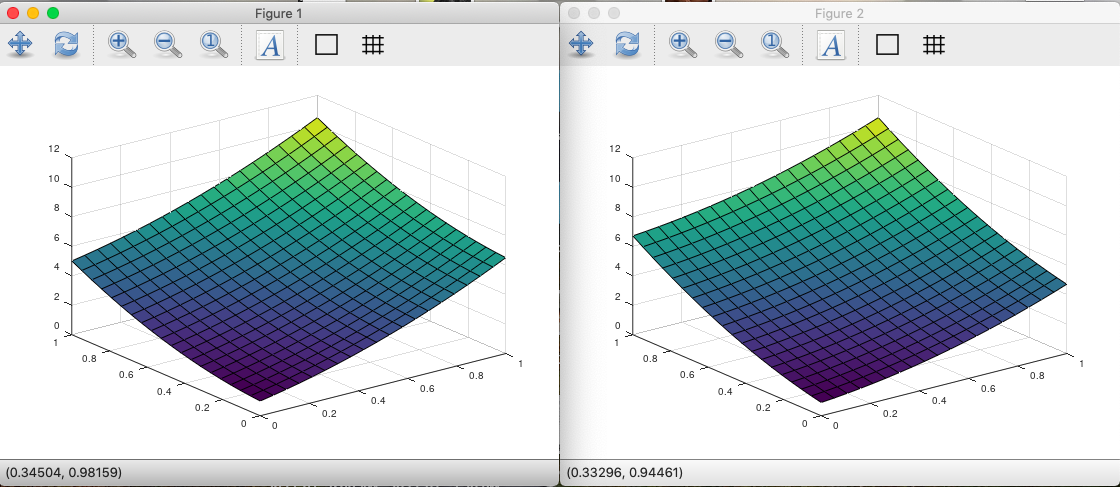
Here’s the finished product, it can optimize N-dimensions, and you can subdivide them however you like. In the attached example, it’s broken into 3 variables and 3 variables, producing a curve in 3 space, but this could also be treated as a single six variable function, and the algorithm is indifferent. The original curve is on the left, the interpolated curve is on the right, and this took just over two minutes to run. The results are awesome. Note you could also use this to find a generalized goal state, as I’ve simply set this example up to find coefficients of a polynomial, but again, the method is generalized. As a consequence, it is a generalized N-Dimensional state space algorithm, that runs very quickly, and has a deterministic runtime, though you are of course not guaranteed any particular results.

I wrote an algorithm that models interference between multiple iterations of the same path. The basic idea is simple: you have a random path, and you generate it some number of times. However, once you traverse a particular location in the path, that point becomes more likely. As a consequence, over time, the probabilities become non-uniform (obviously they start out uniform). When I articulated this, I noted that this is plainly an optimization algorithm, since you can update the probabilities of a given point (treated as a domain value) with the distance to some goal state (in the range). This can done in N-dimensions, by simply having N paths all doing exactly this. Moreover, you can vectorize many of the steps for this N-dimensional case easily in Octave. Here’s the two dimensional code (on dropbox).

Development of Black Tree is complete, for now. As such, I’ve started another Kickstarter Campaign, this time to finance the eventual development of Black Tree Imaging, advertising for the existing products, improvements to the website, and other administrative expenses. Rewards include heavily discounted versions of Black Tree Massive.

I’m thrilled to announce that Black Tree Massive is now for sale on Black Tree’s website, for just $2,999. The performance is ridiculous, as it’s able to classify 30,000 rows in about 3 seconds –

Nothing is even in the same galaxy as my software.

I’ve introduced three algorithms that will form the basis of Black Tree Massive, one is a more efficient but mathematically identical version of my Supervised Delta Algorithm, and the other two are sort-based classification algorithms that have runtimes that completely eclipse even my prior work, which already has unprecedented runtimes, and are themselves almost certainly the fastest algorithms on the market. The Supervised Delta Algorithm is rooted in my paper, Analyzing Dataset Consistency, in which I prove that polynomial time algorithms can produce literally perfect clustering and classification, under certain reasonable assumptions. This typically translates into very high and at times perfect accuracy for benchmark datasets. In another paper, Sorting, Information, and Recursion, I proved a surprising connection between sorting and the nearest neighbor algorithm, specifically, that if a list of vectors is sorted, then the adjacent entries in the sorted list are nearest neighbors of each other (see, Theorem 2.1). As a consequence, if you begin at a given entry in a sorted list, and proceed to adjacent entries in both directions, you will encounter the set of points that are included in some sphere in the Euclidean space of the dataset. This must be true, since the distance between two vectors in a sorted list, can never exceed the sum of the distances over the adjacent pairs that are between them, since this sum is by definition either equal to or greater than the straight-line distance between the two vectors. As a result, you can cluster data by simply collecting vectors in a sorted list, proceeding in both directions, from a given index in the list. Using this method, you don’t have to calculate the norm of the difference between a given vector, and all other vectors in order to find the vectors that are within a given sphere (i.e., within a given radius). This saves significant time during processing, leading to algorithms that can classify at a rate of approximately 4,500 Testing Rows over 25,500 Training rows, in roughly 3 seconds (running on a MacBook Air).

Because the runtimes are so fast, you can therefore run the algorithms hundreds of times, and still produce a practical, and very fast runtime, which in turn allows you to calculate a meaningful measure of confidence that I introduced in yet another paper, Information, Knowledge, and Uncertainty. This process requires running classification a few hundred times in order to generate a distribution of confidence intervals, that are then applied to a final prediction step. Ideally, accuracy should increase as a function of confidence, and this is empirically what happens. This allows you to take the solid raw accuracies produced by the initial sort-based classification algorithms (typically about 80%), and filter predictions, increasing required confidence until you achieve a maximum (or desired) accuracy (typically maximized between 90% and 100%). The net result is very high accuracy, making use of algorithms that can handle simply enormous datasets, running on a consumer device.

This is likely a fundamental breakthrough in computer science, and A.I.

Here are links to notes regarding the algorithms in question, which in each case, includes the relevant Octave code:

Massive Supervised Delta Classification

Massive Supervised Classification

Massive Unsupervised Modal Classification

Attached is the code for the unsupervised analog of the algorithm I presented yesterday. The accuracy seems solid, though it needs more testing, and the runtimes are ballpark the same (i.e., about 10 seconds for 4,500 Testing Rows classified over 25,500 Training Rows).

Attached is the full command line code for the algorithm I mentioned yesterday, which now includes confidence calculations, allowing for higher accuracy. The method is analogous to the ideas discussed in my paper, Information, Knowledge, and Uncertainty [1], in that a confidence metric is assigned to every prediction, and then accuracy is calculated as a function of confidence, though this entire series of algorithms also makes use of sorting, as a faster method to implement a pseudo-nearest neighbor algorithm (see, Theorem 2.1 [2]). What’s interesting is that a much simpler metric for confidence, which is simply the number of elements in the cluster associated with a prediction, works really well, despite not having the same rigorous theoretical basis as the information-based confidence metric I introduce in [1]. This could be because this algorithm is supervised, producing homogeneous clusters (i.e., every cluster consists of a single class), and so you could argue the only relevant factor is the size of the cluster. If this is true, the equation I presented in [1] is wrong, despite the fact that it works, in that there would be another equation that ignores the dataset as a whole, and looks only to the cluster in question. I can’t say whether or not I tested this possibility in the past, and it’s not in my interests to test it now, because I have software that works, and so the academics will have to wait until Black Tree Massive is complete.

As I noted, confidence is calculated for every prediction, in this case twice, once based upon the information metric I introduce in [1], and then again using only the size of the cluster. As you increase confidence, in both cases, you eliminate predictions, leaving some surviving percentage, which is also listed below. The Raw Accuracy is the accuracy prior to filtering based upon confidence, but includes “rejections”, which is a concept from my original algorithms that is carried over here. The runtime of this particular algorithm is simply astonishing, classifying 4,500 testing rows over 25,500 training rows, in about 3 seconds, running on a MacBook Air, which totally demolishes even my prior work, and basically makes a joke of everyone else’s.

Dataset	Raw Accuracy	Max Inf.-Based Accuracy	Surviving Percentage (Inf.)	Max Size-Based Accuracy	Surviving Percentage (Size)
UCI Credit	74.85%	81.01%	0.47%	83.33%	0.60%
UCI Ionosphere	81.32%	85.12%	5.50%	100.0%	0.18%
UCI Iris	97.98%	100.0%	1.36%	100.0%	0.44%
UCI Parkinsons	80.70%	85.16%	24.0%	83.66%	7.30%
UCI Spam	79.00%	80.00%	34.0%	100.0%	0.13%
UCI Wine	80.64%	85.71%	0.50%	96.00%	1.30%