I spend a lot of time thinking about signal and noise, and my intuition is that a signal is something that has a low Kolmogorov Complexity, and noise causes it to have a higher Kolmogorov Complexity. That sounds nice, and I think it makes sense, but the question is, what can I do with this definition? I think the answer so far is nothing, and it’s purely academic. However, it just dawned on me that if noise is statistically random, then it should begin to cancel itself out when it’s sampled independently at a large number of positions. Just imagine pure noise, and sample at different places at the same time – it should either net to zero (additive and subtractive noise), or increase in amplitude (strictly additive noise) as your number of samples grows sufficiently large. This in turn implies that we should be able to discern between true noise, and a signal subject to noise, by increasing the number of independent samples of the ostensible signal. Specifically, if it grows to nothing, or increases in amplitude, without changing structure, then it’s pure noise. If it instead changes structure, then it suggests that there is an underlying signal, subject to additive and subtractive noise that is starting to net itself out. In contrast, I don’t think there is any obvious solution to strictly additive noise. Nonetheless, this is a pretty good practical definition of signal versus noise, that definitely works, and I just wrote some simple code in Octave where you increase the number of independent noisy representations of a signal, and the average plainly reduces noise, as a function of the number of independent representations.

Some of my recent work suggests the possibility that genetic sequences are locally consistent, in that small changes to bases do not change macroscopic classifiers (e.g., species, common ancestry, and possibly even traits). I’m still testing this empirically, but I’ve already developed an algorithm that produces perfect accuracy on an NIH Dataset I put together from Influenza A and Rota Virus samples. The classification task was in that case really simple, simply distinguishing between the two species, but the accuracy was perfect. I only used 15 rows of each species, and it was literally perfect.

I also tested it on three datasets from Kaggle, that contain different genetic lines of dogs, chimpanzees, and humans. The classification task in that case is to predict the subclass / family line of each species, given its genetic base data. This is a tougher classification because you’re not distinguishing between species, and instead you’re identifying common family lines within each species.  Accuracy peaked at perfect for all three, which is expressed as a function of confidence. For the NIH dataset it was perfect without confidence filtering. The method I’ve employed in all cases is a simple modification of the Nearest Neighbor algorithm, where sequences x and y are treated as nearest neighbors if x and y have the largest number of bases in common over the dataset of sequences. This implementation is however highly vectorized, resulting in excellent runtimes, in this case fully processing a dataset with 817 rows and 18,908 columns in about 10 to 12 seconds. There is then a measure of confidence applied that filters predictions.

I will continue to test this algorithm, and develop related work (e.g., a clustering algorithm follows trivially from this since you can pull all sequences that have a match count of at least k for a given input sequence). Here’s a screen shot for the Kaggle dog dataset, with the number of surviving predictions as a function of confidence on the left, and the accuracy as a function of confidence on the right:

Attached is the code, subject to my stated Copyright Policy (as always).

I’m currently working on genetics, and already came up with some novel algorithms that I think are interesting, but are not yet empirically tested. I did however, out of curiosity, simply assign the numbers 10,11,12,13 to the bases A,T,G,C, respectively, and ran Black Tree’s Supervised Delta Algorithm on a dataset from Kaggle, that contains dog DNA, and the accuracy was 82.6%, using a simply minuscule percentage of the basepairs in the dataset, which is quite large. Specifically, I used 30 bases from the dataset, which for some rows contained 18,908 bases. Yet again, this software outperforms everything else by simply gigantic margins. The runtime was 0.31 seconds, running on a cheap laptop. You can do a limited version of exactly this using the totally Free Version of Black Tree AutoML, that will let you run Supervised Delta on just the training dataset (i.e., there’s no training / testing for free). My next step will be to optimize the values assigned to the bases, which are obviously not meaningful, and I have an optimization algorithm that can do exactly that. Here’s a screen shot of the output using Black Tree Massive:

 

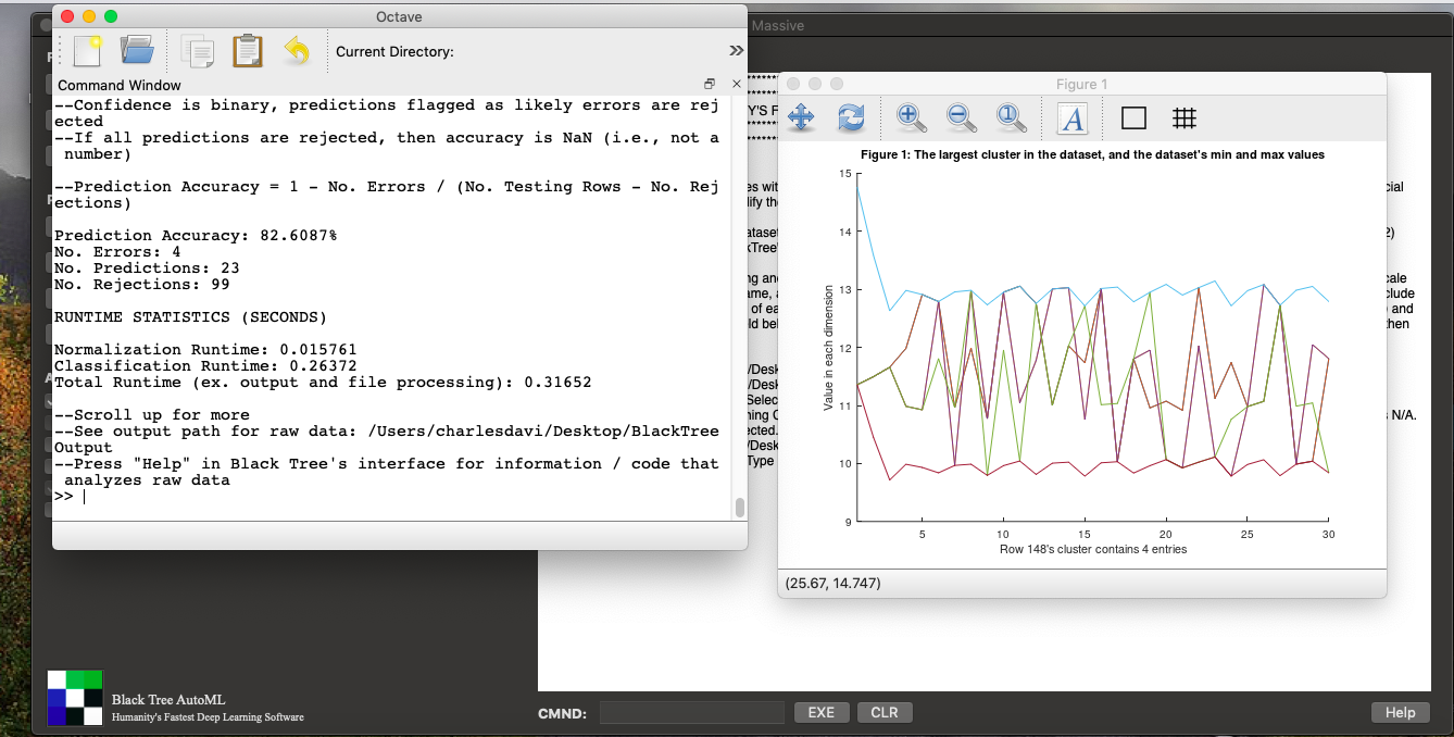
Here are the datasets (dog_training, dog_testing), simply download and run Black Tree on these, though again, the Free Version will limit you to just the training file. I’m still hunting down the provenance of the dataset, because it is Kaggle and not a primary source, but if this is a bona fide dataset, it would be evidence for the claim that DNA is locally consistent. If that is true, then my existing software (and other simple methods such as Nearest Neighbor) will as a general matter perform, which means there’s really no reason to do much more work on the topic. This would allow researches to focus on identifying genes and classifying populations, and developing therapies.

I’ve written a simple delimiter algorithm that allows you to delimit genetic sequences. The basic idea is, if a base is sufficiently dense at an index in a population, then it could be part of a gene, and so a sequence of sufficiently dense bases in order, is therefore useful to identify, since that sequence of bases could therefore form a gene.

The basic idea for this algorithm is really simple: calculate the densities of the bases in a population, at each index in a sequence, then calculate the standard deviation of those densities.

Now read the densities in the order of the underlying genetic sequence, and if you see the density change by more than the standard deviation, mark that index with a delimiter. So if e.g., the standard deviation is 20%, and there’s a jump from 90% density to 50% density, then you put a delimiter between the 90% and 50% dense bases, marking the end of a gene.

All of the operations in the code can be run in parallel, and so it has a constant runtime, on a parallel machine. It is extremely fast even running on an ordinary laptop.

Here’s a more detailed example:

The bases are assumed to be pulled from a single strand of DNA, since the pairs are determined by one strand. The example in the code below uses a population of 100 people, each with 50 bases, creating a matrix with 50 rows (i.e., the number of bases per individual) and 100 columns (i.e., the number of individuals in the population). The next step is to find the modal base for each row, which would be the most frequent base at a given index in a sequence. Let’s assume for example there are 80 A’s and 20 G’s, in a given row. The modal base is A, and the density is 80%. We do this for every row, which will create a column vector of densities, with one entry / density for each row of the matrix. Now you read that vector in order, from index 1 to N, and if the transition from one row to the next changes by more than the standard deviation of the densities, you mark a delimiter between those two indexes.

So let’s assume the densities between two rows transition from 80% to 50%, and the standard deviation is 20%. We would mark a delimiter between those two rows, indicating the end of a gene, because we went from a base that many had in common, to a base that few had in common. The tacit assumption being, that genes will be common to a population, indicating signal, and everything else will be noise. By delimiting in this manner, we indicate the end of a gene and the commencement of noise.

Here’s the code:

https://www.dropbox.com/s/zo0x1u46qbt2fci/Genetic%20Delimter%20CMNDLINE.pdf?dl=0

 

Following up on a previous post where I introduced an algorithm to find the longest genetic sequence common to a population, I’ve now applied my most basic clustering algorithm to genetic sequences, in order to classify populations based upon genetic data, and the results are excellent, at least so far, and I’d welcome additional datasets to test this on (my software is linked to below).

The basic idea is to use A.I. clustering, to uncover populations in genetic data. 

To test this idea, I created two populations, each based upon a unique genetic sequence that is 50 base pairs long, and each sequence was randomly generated, creating two totally random genetic sequences that are the “seeds” for the two populations. Each population has 100 individuals / sequences, and again, each sequence is 50 base pairs long. This ultimately creates a dataset that has 200 rows (i.e., individuals) and 50 columns (i.e., base pairs).

I then added noise to both populations, randomizing some percentage of the base pairs (e.g., swapping an A with a T). Population 1 has 2.5% of its base pairs effectively mutated using this process, and Population 2 has 5.0% of its base pairs mutated. This creates two populations that are internally heterogenous, due to mutation / noise, and of course distinct from one another (i.e., the original sequence for Populations 1 and 2 were randomly generated and are therefore distinct).

The A.I. task is to take the resultant dataset, generated by combining the two populations into a single dataset, and have the algorithm produce what are called “clusters”,  which in this case means that the algorithm looks at the genetic sequence for an individual, and pulls all other sequences that it believes to be related to that individual, without “cheating” and looking at the hidden label that ultimately allows us to calculate the accuracy of the algorithm.

The algorithm in question is interesting, because it is unsupervised, meaning that there is no training step, and so the algorithm starts completely blind, with no information at all, and has to nonetheless produce clusters. This would allow for genetic data to be analyzed without any human labels at all.

This is in my opinion quite a big deal, because you wouldn’t need someone to say ex ante, that this population is e.g., from Europe, and this one is from Asia. You would instead simply let the algorithm run, and determine on its own, what individuals belong together based upon the genetic information provided, with no human guidance at all.

In this case, the accuracy is perfect, despite the absence of a training step, which is actually typical of my software, and there’s a set of formal proofs I presented that guarantee perfect accuracy under reasonable conditions, that are of course violated in some cases, though this (i.e., genetic datasets) doesn’t seem to be one of them. However, I’ll note that the proofs I presented (and linked to) relate to the supervised version of this algorithm, whereas I’ve never been able to formally prove why this algorithm works, though empirically it most certainly works across a wide variety of datasets. It is however very similar to the supervised version, and you can read about the supervised version here.

Finally, I’ll note that because there are only 4 base pairs, the sequences are relatively short (i.e., only 50 basepairs long), and they’re randomly generated with random noise, it’s possible to produce disastrous accuracy, using my model datasets. That is, it’s possible that the initially generated population sequences are sufficiently similar, and then noise makes this problem even worse, producing a dataset that doesn’t really have two populations. And for this reason, I welcome real world datasets, as I’m new to genetics, though not new to A.I.

Begin with a sequence of DNA base pairs for each individual in a population of size . Then separate these sequences into single strands of DNA. Assume that each DNA strand contains individual bases over . Now construct a matrix where each column of contains characters that define the DNA sequence of exactly one individual from the population. It follows that is a matrix with rows (i.e., the number of bases) and columns (i.e., the number of individuals in the population). You can think of the matrix as readable from the first row of a given column, down to the bottom row of that same column, which would define the genetic sequence for a given individual in the population.

Now construct a new matrix such that , where maps to . That is, maps each of the four possible bases to the numbers 1 through 4, respectively. All we’ve done is encode the bases from the original matrix using numbers. Now for each row of , calculate the density of each of the four bases in the row, and store those four resultant densities in a matrix , that has rows and columns. That is, each of the four possible bases will have some density in each row of , which is then stored in a corresponding row of , with each of the four columns of containing the densities of , respectively, for a given row of .

Further, construct a vector with a dimension of , where row of contains the maximum entry of row of . That is, for every row of , which contains the densities for each of the four bases over every row, we find the base that is most dense for a given row, and store that density in the corresponding row of a new vector . Then, construct a binary vector that maps every element of to either or , depending upon whether or not the entry in question is greater than some threshold in . The threshold allows us to say that if e.g., the density of A in a given row exceeds , then we treat it as homogenous, and uniformly A, disregarding the balance of the entries that are not A’s. It follows that the longest sequence of consecutive in , is the longest sequence of bases common to the entire population in question (subject to the threshold). All of these operations have in the worst case a linear runtime, or less when run in parallel. As a consequence, we can identify DNA sequences common to an entire population in worst case linear time.

The first step of mapping the bases to letters can be done independent of one another, and so this step has a constant runtime in parallel. The second step of calculating the densities can be accomplished in worst case linear time, for each row, since a sum over operands can be done with at most operations. The densities for each row can be calculated in parallel, and so this step requires a linear number of steps as a function of . The next step of taking the maximum densities can again be done in parallel for each row, and requires operations for a given row. The next step of comparing each maximum density for each row to a fixed threshold can again be done in parallel, and therefore requires constant time. The final step of finding the longest sequence requires exactly operations. As a result, the total runtime of this algorithm, when run in parallel, is .

Attached is Octave code that implements this, and finds the longest genetic sequence common to a population (using the threshold concept). This can be modified trivially to find the next longest, and so on. This will likely allow for e.g., long sequences common to people with genetic diseases to be found, thereby allowing for at least the possibility of therapies.

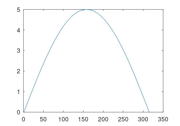
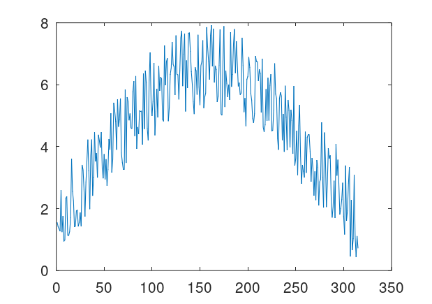
Quantize a space of amplitudes to achieve a code. That is, each one of finitely many peak amplitudes corresponds to some symbol or number. So if e.g., a signal has a peak amplitude of 4, then the classifier / symbol it encodes is 4. Now posit a transmitter and a receiver for the signals. Send a signal from the transmitter to the receiver, and record both the known peak amplitude label transmitted (i.e., the classifier), and the received amplitudes at the receiver. Because of noise, the transmitted amplitudes could be different from the received amplitudes, including the peak amplitude, which we’re treating as a classifier. For every given received signal, use A.I. to predict the true transmitted peak amplitude / classifier. To do this, take in a fixed window of observations around each peak, and provide that to the ML algorithm. The idea is that by taking a window around the peak amplitude, you are taking in more information about the signal, rather than just the peak itself, and so even with noise, as long as the true underlying amplitude is known in the training dataset, all transmitted signals subject to noise should be similarly incorrect, allowing an ML algorithm to predict the true underlying signal. Below is an original clean signal (left), with a peak amplitude / classifier of 5, and the resultant signal with some noise (right). Note that the amplitudes are significantly different, but nonetheless my classification algorithms can predict the true underlying peak amplitude with great accuracy, because the resultant noisy curves are all similarly incorrect. Note that the larger the set of signals, the more compression you can achieve, since the number of bits required reduces as a function of the base of the logarithm, , where is the number you’re trying to encode. The datasets attached use 10 signals, with peak amplitudes of 1 through 10.

Attached is code that generates datasets, simply run Black Tree on the resultant datasets. The accuracies are very high, and it’s perfect for one way additive noise up to about 225% noise. For two-way noise (additive and subtractive), the accuracies are perfect for 25% noise, and about 93% for 100% noise. The noise is calculated as a real number, since the maximum amplitudes are have a distance of 1 from each other. So a noise level of 100% means that the transmitted amplitude can differ from the true underlying amplitude by at most 1. You could also do something analogous with frequencies (e.g., using fixed duration signals), though amplitude seems easier since you can simply identify peaks using local maximum testing (i.e., amplitude goes up then down), or use a fixed duration.

This process could allow for communication over arbitrary distances using inexpensive and noisy means, because you can achieve literally lossless transmission through the use of prediction. Simply include prediction in repeaters, spaced over the distance in question. And because Black Tree is so simple, it can almost certainly be implemented using hardware. So the net idea is, you spend nominally more on repeaters that have predictive hardware in them, and significantly less on cables, because even significant noise is manageable.

The density of a system could be non-uniform. Just imagine a baseball with feathers glued to its surface. If someone throws that baseball at you, getting grazed by the feathers is a fundamentally different experience than getting hit with the ball itself. This seems trivial and obvious, but it implies something interesting, which is that the density of a system could easily be non-uniform, and as a consequence, its momentum would in that case also be non-uniform. This is why getting grazed by the feathers is preferable, simply because they have less momentum than the body of the ball itself, despite the system moving as a whole, with a single velocity. As a general matter, this observation implies that interactions between materials, including mediums like air, could be locally heterogenous, despite the appearance of uniformity.

A second and not entirely related note is that all materials make use of free energy from fields. This must be the case, for otherwise gravity would cause everything to collapse to a single point. This does not happen because of intramolecular forces, that are the result of free energy from fields. This is again an obvious-in-hindsight observation, but it’s quite deep, for it implies that the structure of our Universe is due to the free energy of fields. That there’s a constant tension between the force of gravity and the intramolecular and atomic forces at work in literally every mass.

It just dawned on me that we might be able to cure diseases associated with individual genes that code for specific proteins, by simply suppressing the resultant mRNA. This could be accomplished by flooding cells with molecules that are highly reactive with the mRNA produced by the “bad gene”, and also flooding cells with the mRNA produced by the correct “good gene”. This would cause the bad gene to fail to produce the related protein (presumably the source of the related disease), and instead cause the cell to produce the correct protein of a healthy person since they’re given the mRNA produced by the good gene.

I noted in the past that a UTM plus a clock, or any other source of ostensibly random information, is ultimately equivalent to a UTM for the simple reason that any input can eventually be generated by simply iterating through all possible inputs to the machine in numerical order. As a consequence, any random input generated to a UTM will eventually be generated by a second UTM that simply generates all possible inputs, in some order.

However, random inputs can quickly approach a size where the amount of time required to generate them iteratively exceeds practical limitations. This is a problem in computer science generally, where the amount of time to solve problems exhaustively can even at times exceed the amount of time since the Big Bang. As a consequence, as a practical matter, a UTM plus a set of inputs, whether they’re random, or specialized to a particular problem, could in fact be superior to a UTM, since it would actually solve a given problem in some sensible amount of time, whereas a UTM without some specialized input would not. This suggests a practical hierarchy that subdivides finite time by what could be objective scales, e.g., the age of empires (about 1,000 years), the age of life (a few billion years), and the age of the Universe itself (i.e., time since the Big Bang). This is real, because it helps you think about what kinds of processes could be at work solving problems, and this plainly has implications in genetics, because again you’re dealing with molecules so large that even random sources don’t really make sense, suggesting yet another means of computation.