Attached is code that implements an analog of my core supervised classification algorithm to genetic sequences. The original algorithm operates on Euclidean data, and because genetic sequences are discrete, this algorithm simply increases the minimum matching number of bases between two sequences, rather than increasing a spherical volume of Euclidean space. You can read about the original algorithm in my paper, Vectorized Deep Learning, and this works exactly the same way, it’s just not Euclidean. I tested it on three datasets from Kaggle, that contains raw genetic sequences for dogs, humans, and chimpanzees, the classification task being to identify common ancestor classes, separately, for each species (i.e., it’s three independent datasets). The accuracy was roughly 100% for all three datasets. The runtimes were 78 seconds (695 training rows, 122 testing rows, 18,907 columns); 371.314 seconds (1,424 training rows, 251 testing rows, 18,922 columns); and 1,752 seconds (3,085 training rows, 544 testing rows, 18,922 columns), respectively. This is consistent with how this algorithm performs generally, as it is extremely efficient and highly accurate. The only difference here is that the data is not Euclidean. This is more empirical evidence for the claim that genetic data is locally consistent, which in turn implies that polynomial-time algorithms can be used to accurately classify genetic data.

 

The Shannon Entropy is not a good measure of structural randomness, for the simple reason that all uniform distributions maximize the Shannon Entropy. As a consequence, e.g., a sequence of alternating heads and tails maximizes the Shannon Entropy, despite having an obvious structure. The Kolmogorov Complexity solves this, since the shortest program that generates an alternating sequence of heads and tails is obviously going to be much shorter than the length of the sequence, and therefore such a sequence is not Kolmogorov-Random, which requires the complexity to be the length of the sequence plus a constant.

However, Kolmogorov Randomness is too strong of a requirement, since there are sequences that are intuitively random, that are not Kolmogorov Random. Specifically, consider e.g., a Kolmogorov Random string . Now partition that string into substrings . This collection of substrings must also be Kolmogorov Random, for assuming otherwise implies that we can compress , which contradicts our assumption that is Kolmogorov Random. We can then interpret each as a binary number. Now construct a new binary string , such that consists of 1’s, in a sequence, followed by a 0, then 1’s, in a sequence, followed by a 0, etc. That is, is constructed by treating each as the length of a sequence of 1’s, that is followed by a 0. We can therefore specify by specifying each , which requires bits. As a consequence, if , then simply specifying each sequence length will compress . Nonetheless, sequence is intuitively random, because the indexes of the 0’s are given by a Kolmogorov Random string. However, if the numbers encoded by each are sufficiently large, then could be significantly less than , and as such, would not be Kolmogorov Random.

This suggests a simple and intuitive definition of a random string, where a string is random if . That is, if the subsequences of a string cannot be compressed beyond identifying their lengths, then the string is random, even though it is not Kolmogorov Random. Note that it doesn’t matter whether we identify the 0’s or 1’s in a string, since we can simply take the complement of the string, which requires an initial program of constant length that does not depend upon the string, thereby increasing the Kolmogorov Complexity by at most another constant.

This is quite nice, because it’s simple, and it allows for sequences that have arbitrarily long periods of stability to still be treated as random. And as a consequence, if a sequence has an extremely low entropy, it could still be random in this view, if its subsequences cannot be compressed beyond identifying their lengths.

I published some code that iteratively applies Nearest Neighbor until you create a loop. That is, you run Nearest Neighbor on its on output until you return the same row twice. Symbolically, if is our initial input, and is the Nearest Neighbor of , we repeatedly calculate until some . This creates clusters, which could be useful on its own, though it also defines quantized distances between the elements of the dataset, since the repeated application of Nearest Neighbor connects rows through a path, and so the quantized distance between two rows in a dataset is simply the number of edges that separate them. That is, and are separated by a distance of .

But it just dawned on me, if you don’t allow it to create a loop, and instead delete any row that produces a loop, and apply it again, until you find a unique output, it will force you to iterate through the entire dataset, quantizing the distance between a given starting row, and all other rows. If you do this for a population of genetic sequences, e.g., using human genomes, you can then define the distance between a member of a given population, and all other populations, globally. If you do this repeatedly, you will create a distribution of distances from one population to all others. So if for example you start with a large group of Chinese people, and then apply Nearest Neighbor, using a subset of the entire world population as your dataset (i.e., all major geographies), you will construct a quantized distribution of distances from Chinese people to all other people, which will of course probably iterate through a large number of Chinese people before moving on, but it will eventually move on.

This distribution will also of course create averages, allowing you to say that, e.g., on average Chinese people are a quantized distance of one, two, etc., from populations A,B, and so on. It will also allow you to identify anomalies, since everyone will fall within that distribution, at some distances from the averages. This is now doable, because of the IGSR Dataset, and I’m just starting to download files, which are extremely large, so this will take some time.

If you can figure out a mapping across species, you could in theory apply this process to the entire set of known organisms, creating a distance metric that covers all species.

Fields are plainly a source of free energy, in that e.g., gravity can cause arbitrary blue shifting in photons, and arbitrary acceleration in masses. You can fuss about Potential Energy, but it’s nonsense, especially in the case of a photon, that literally gains Kinetic Energy that was not there before through blue shifting. The more sensible theory of Potential Energy, is that when it is present in a system, it is actually Kinetic Energy that causes no macroscopic motion, and instead causes only small scale motions that must on average “net out” to nothing at the macroscopic level.

Biological life plainly makes use of fields, beyond the obvious of our nervous system, and instead it is a fundamental part of the storage and use of energy in even bacteria, where small scale differences in charges drive molecular machines that, e.g., allow for the production of ATP:

As a consequence, if it’s possible to extract more energy through fields than is consumed through e.g., combustion, then life itself should have figured out how to do this by now, since there is to our knowledge, no laboratory that’s been around for longer than life itself. The general idea being that because it would be advantageous to extract more energy from a field than is consumed in accessing the field, and because the Earth is so large and diverse, and old, it should have occurred by now. This should be measurable, but it would likely require careful, comprehensive, and invasive measurement of all energy consumed by and produced in an organism.

Note that this does not imply perpetual energy, and instead implies that a small bang (from e.g., combustion) is then followed by a bigger bang (from e.g., an electrostatic field), causing the entire process to have a positive yield. This second production of energy might not be translatable back into e.g., chemical energy, and so no infinite loop is necessarily produced by such a process. That said, if it actually turns out that some life generates more energy than it consumes, then it is obviously worthy of study, since human beings might able to adapt these processes into energy producing systems, that would by definition be more efficient than e.g., combustion alone. The general mechanical intuition being that you use chemical energy, or mechanical energy, to access the free energy of some field, likely magnetic, or electrostatic, but anything is possible, what works is what matters.

I’ve posited that anti-gravity is the force that keeps one moment in time from intruding into another, and this makes perfect sense, since it completes the symmetry of gravity, and would force integrity on time itself, preventing the future, past, and present from interacting, as a general matter, though it’s obviously a highly speculative idea. I’ve also speculated that it’s not perfect, which would allow for small scale, spontaneous particles and energy to appear without any ultimate cause, with some low probability, which from what I remember, is what actually happens.

The other day I realized that this could be used to explain Quantum Interference, though I’ll concede at this point, I’ve introduced a number of theories for this phenomenon. The basic idea is that a particle literally interferes with its most proximate moment in the future, causing it to behave as if there were a multitude of instances of itself. In this view, this should not happen as often as particles get larger, and that is plainly true at our scale of existence, where this literally never happens.

However, there’s one problem with this theory, which is that the introduction of e.g., an intervening particle destroys the interference pattern generated by the Double Slit Experiment. However, we can remedy this by observing that exchanges of momentum plainly do not cause this to happen, because e.g., the walls that define the experiment are plainly in the scope of the path of the particle, yet their presence does not destroy the interference pattern. As a consequence, we can posit that exchanges of momentum alone that do not change the energy of a particle, do not destroy the interference pattern, and therefore do not change the path of the particle through time, allowing it to still interact with future instances of itself.

We can then also posit that a change in energy (e.g., one caused by the introduction of an intervening particle that collides with the original particle), does change the path of the particle through time, thereby preventing it from interacting with what were otherwise future instances of itself.

The question still remains, what can cause something to transition from a point particle, to a wave? I haven’t really studied physics in years, but I was pretty thorough when I did, and I don’t recall seeing this question answered. So this is no worse off than a Copenhagen interpretation that posits what is basically the diffusion of the energy of a particle over multiple possibilities in one moment in time, and this was in fact my original theory:

https://www.researchgate.net/publication/344047683_A_Combinatorial_Model_of_Physics

The difference here is that we should be able to test whether or not there is in fact unexplainable interference happening generally, at extremely small scales, and I believe this has in fact been observed. Such an occurrence has nothing to do with Quantum Interference, and instead requires a totally separate assumption, and I guess you could invoke the Uncertainty Principle. Though if both explain the same set of observations, and one is universal, requiring a single assumption, instead of two, then it’s a stronger axiom.

One final note, this implies that true acceleration, i.e., a change in energy, not momentum alone (e.g., simply turning the wheel without pressing the gas), does not change the path through time, suggesting that time itself contemplates or connects possibilities that are connected through a single level of energy.

When you have a known set or population generally, with some known measurable traits, it’s a natural tendency to attribute the properties of that set, to new observations that qualify for inclusion in that set. In some contexts, this is deductively sound, and is not subject to uncertainty at all. For example, we know that the set of prime numbers have no divisors other than themselves and . And so as a consequence, once we know that a number is included in the set of prime numbers, then it must be the case that any property that applies to all prime numbers, also applies to this new prime number. However, observation of course goes beyond mathematics, and you could for example be dealing with a population of genomes, with some known measurable property. Now given a new genome that qualifies for inclusion in this population, how can we be sure that the property of the population also holds for the new observation? There is no deductive reason for this, and instead it is arguably statistical, in that we have a population with some known property, which is universal in the known population, and we have some new observation that qualifies for inclusion in that population, under some criteria. Even if the criteria for inclusion in the population is directly measurable in the genome itself (e.g., an A at index ), you cannot be sure that the property actually holds, unless it follows directly from that measurement. More generally, unless inclusion in a given set is determined by a given measurement, and the property asserted of all elements in the set follows deductively from that measurement, you cannot with certainty attribute that property to some new observation.

Put all of that aside for a moment, and let’s posit some function that allows you to generate a set, given a single element. If that function truly defines and generates a unique set, then applying that function to the elements of the generated set, should not produce new elements, and should instead produce exactly the same set. Said otherwise, it shouldn’t matter what element I start with, if our function defines a unique set. To create a practical example, view the set in question as a cluster taken from a dataset. This is quite literally a subset of the dataset. There must be in this hypothetical a function that determines whether or not an element of the dataset is in a given cluster. Let’s call that function , and assume that is either or , indicating that the element is either not in the cluster, or in the cluster, associated with element , respectively. That is, , when applied to all in the dataset, will generate a cluster for . Now for each in the cluster associated with , calculate over all in the dataset. This will generate another cluster for every element of the original cluster associated with .

For each such cluster, count the number of elements that are included in the original cluster associated with . The total count of such elements, is a measure of the inter-connectedness of the original cluster associated with , since these are the elements that are generated by our function, given a new starting point, but are not new. Now count the number of elements that are not included in the original cluster associated with , these are new elements not in the original cluster. Viewed as a graph, treating each element of the original cluster for as a vertex, we would then have a set of edges that mutually connect elements of the original cluster for , and then a set of edges that go outside that cluster. If there are no edges coming out of the original set of elements in the cluster for , then defines a perfectly self-contained set, that will always produce the same set, regardless of the element that we start with. More generally, you’re producing an analogous set for each element of a given set. Intuitively, the more self-contained that original set is, under this test, the more confident we are that the properties of the elements of that set are attributable to elements that qualify for inclusion in that set, for the simple reason that it is disconnected, quite literally, from all other sets. If a set is not self-contained, then it is by definition associated with other sets that could have other properties.

We can make this rigorous, using the work I presented in, Information, Knowledge, and Uncertainty [1]. Specifically, your intuitive uncertainty in the attribution of properties of a set to new observations that qualify for inclusion in the set, increases as a function of the number of outbound edges. Similarly, your intuitive uncertainty decreases as a function of the number of mutually connective edges. We can measure uncertainty formally if we can express this in terms of the Shannon Entropy. As such, assign one color to the edges that are mutually connective, and assign a unique color for every other remaining vertex (i.e., element of the set). So if an element of the original cluster for connects to some external element , then the edge connecting to will have a unique color assigned to . As such, all edges that connect to will have the same color. If instead connects to another element of the original cluster , then it will have a different color, that is common to all mutually connective edges. As such, we will have two categories of colors, one color for all mutually connective edges, and a set of colors for all outbound edges. This will create a distribution of colors. Take the entropy of that distribution, and that will be your Uncertainty, . So if for example, all of the edges are mutually connective, they will have a single color, and therefore an entropy and Uncertainty of . Let be the total number of edges, i.e., mutually connective and outbound edges, and let be the number of edge colors. Information is in this case given by (See, [1] generally). Knowledge is then simply .

One interesting note, that comes up every time I’ve worked on epistemology, is that if these results are empirically true (and as it turns out the results in [1] are in fact empirically true), it implies that our theory of knowledge itself is subject to improvement, separate and apart from the knowledge we obtain from experiment and deduction. This branch of what I suppose is philosophy therefore quantifies the knowledge that we obtain from empirical results. This study seems similar to physics, in that the results are axiomatic, and then empirically tested. In contrast, mathematical knowledge is not subject to uncertainty at all. And as a result, this work suggests that empiricism requires the careful and empirical study of knowledge itself, separate and apart from any individual discipline. Said otherwise, this work suggests, that empiricism is itself a science, subject to testing and improvement.

Attached is a clustering algorithm specific to genetics. It pulls all genomes that have a minimum number of K matching bases in a dataset, with respect to a given input sequence. This algorithm is mentioned in this paper. There’s an additional segment of code that is based upon my unsupervised clustering algorithm that generates a value of K for you.

Also attached is an algorithm that analyzes the inter-connectivity of a cluster. Specifically, it’s hard to find circuits and other structures in graphs, so as a workaround, this algorithm simply takes the union of the rows in a sequence of clusters, and tracks the rate of change in the number of elements. So for example, if the first cluster contains 400 elements, and the next row contains 410 elements, only 10 of which are novel, then the total cardinality of the union will be relatively unchanged by 10. By tracking this rate of change we get a measure of the interconnectivity of a sequence of clusters.

Two more methods in genomics I wanted to share, the first being a simple measure of signal versus noise rooted in my work on epistemology. The second is a clustering algorithm I came up with a long time ago but never implemented, rooted in the Nearest Neighbor method.

Assume your population is stored as an matrix, with sequences, and bases per sequence. Now assume we measure the density of each of the four bases in column i. If it turns out that the densities are given by for A,C,G,T, respectively, it’s reasonable to conclude that the modal base of A with a density of 0.9 is signal, and not noise, in the sense that basically all of the sequences in the dataset contain an A at that index. Moreover, the other three bases are roughly equally distributed, in context, again suggesting that the modal base of A is signal, and not noise.

When you have a continuous signal, noise is easier to think about, because if it’s both additive and subtractive, it should cancel itself out through repeated observation. A population drawn from a single species is analogous, because you are in effect repeatedly sampling some “true” underlying genetic sequence, subject to mutations / noise. Unfortunately, you cannot meaningfully take the average of a discrete signal sequence like a genome. However, this doesn’t change the fact that a uniform distribution is indicative of noise. So if for example, the densities were instead , then we could reasonably dismiss this index as noise, since the bases are uniformly distributed at that index across the entire population. In contrast, if we’re given the densities , then we should be confident that the A is signal, but we should not be as confident that the C is noise, since the other two bases both have a density of 0.

We can formalize this by applying the measures of Information, Knowledge, and Uncertainty I presented in the paper of the same name. Information is in this case the applicable maximum entropy, which is for all four bases, for three bases, etc. Uncertainty is is the entropy of the distribution, and Knowledge is the balance of Information over Uncertainty, . Interestingly, this suggests an equivalence between Knowledge and signal, which is not surprising, as I’ve defined Knowledge as, “information that reduces uncertainty.”

I also wrote an interesting clustering algorithm that keeps applying Nearest Neighbor in a chain, until it hits a loop. So for example, first we find the Nearest Neighbor of row i, let’s say it’s row j. Then we find the Nearest Neighbor of row j, and keep doing this until we create a loop, by returning the same row more than once. I haven’t tested it too much, but it seems meaningful because the clusters are generally very small, suggesting that it’s not flying around the dataset, and is instead pulling rows that are proximate to each other.

 

I’m continuing to work on the applications of Machine Learning to Genomics, and my work so far suggests that genetic sequences are locally consistent, in that the Nearest Neighbor method generally produces good accuracy. More importantly, the Nearest Neighbor of a given sequence seems to be determined by only a fraction of the total sequence. Specifically, if we sample a random subset of the bases, and increase the size of that subset, sequences quickly converge to their true Nearest Neighbor. That is, even if we use only a fraction of the bases, the Nearest Neighbor method returns the true Nearest Neighbor that would be found if we used all of the bases. This is surprising, and is consistent with the hypothesis that bases are not truly random. Specifically, this is consistent with the hypothesis that a small number of bases, determines some larger number of bases. The attached code randomly selects an increasing number of bases, and applies the Nearest Neighbor method. Because the base indexes are randomly selected, it suggests that every subset of a sequence partially determines some larger sequence.

If this is true, then genetic sequences are not truly random. If they are not truly random, how do we explain the diversity of life, even given the amount of time in play? Note that this would not preclude randomized mutations to individual bases, but it does suggest that a sizable number of randomized mutations will cause an even larger sequence to mutate. 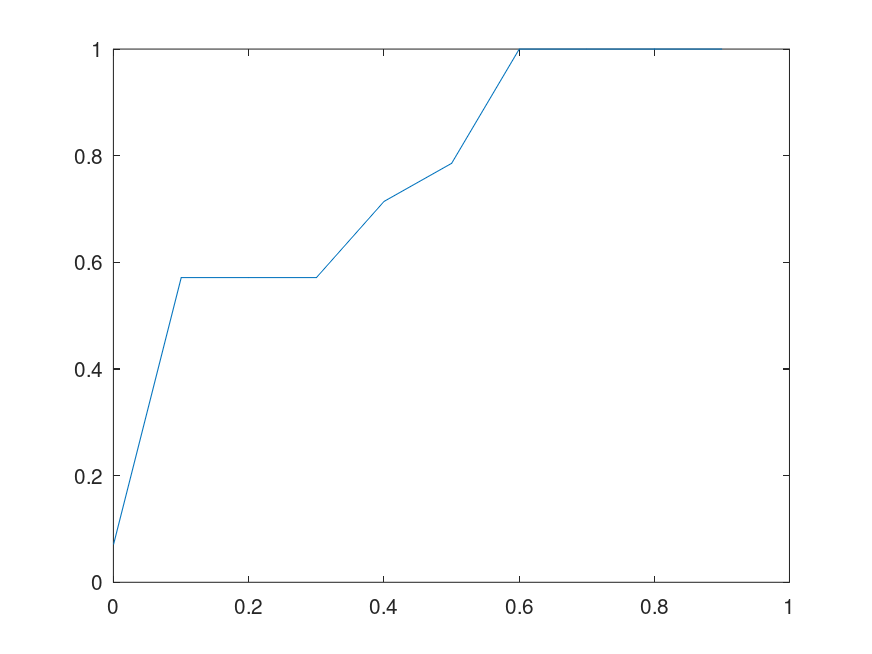Below is a plot of the percentage of sequences that converge to their true Nearest Neighbor, given of the bases in the full sequence (i.e., the horizontal axis plots the percentage of bases fed to the Nearest Neighbor algorithm). The plot on the left uses the genome of the Influenza A virus, and the plot on the right uses the genome of the Rota virus. Both are assembled using data from the National Institute of Health.

This brings genetic sequences closer to true computer programs, because in this view, not all sequences “compile”, and as a consequence, if two sequences match on some sufficiently large but sufficiently incomplete number of bases, then they should match on an even larger subset of their bases, since the matching subset fixes some larger subset of the bases. This would allow for partial genetic sequences to be compared to datasets of complete genetic sequences, potentially filling in missing bases. If this is true, it also casts doubt on the claim that the diversity of life is the product of random and gradual changes, since the number of possible base-pairs is simply astronomical, and if most of the possible sequences don’t code for life, as a result of possibility being restricted by selection, you’ll never get to life in any sensible amount of time, because all the sequences that contain prohibited combinations will be duds, and not persist, thereby cutting short that path through the space of possible sequences. In other words, this would require luck, to simply land at the correct mutations, rather than gradually arriving at the correct mutations in sequence.

We can resolve this by allowing for both small-scale mutations, and large-scale mutations, which could lead to drastic changes in measurable traits. In other words, this doesn’t preclude evolution, it simply requires evolution to be extremely subtle (i.e., some small number of bases mutate), or drastic (i.e., some large number of bases all change together). In summary, if this is true, then mutations are either small in number, or sufficiently large in number, causing an even larger sequence to change, generating either duds, or traits that are permitted. Natural Selection would then operate on the traits that are permitted, allowing the environment to determine what traits persist in the long run.

I’ve assembled my recent work on genetics into a single article, “Vectorized Computational Genomics“. Code is included.