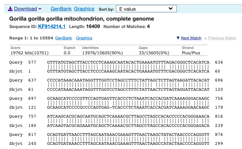
I ran an algorithm on the full dataset that finds the best global alignment when comparing two genomes. I applied this to a complete Heidelbergensis mtDNA genome, comparing it to all other mtDNA genomes in the dataset below (405 complete genomes), and it turns out, you get exactly the same population using the default NIH alignment. See Section 1.3 of Vectorized Computational Genomics [1], for a discussion of the default NIH alignment. Note that the acronyms for the population names in the graphs below can also be found at the end of that paper. Specifically, on the left below is the distribution of genomes that are at least a 96% match with Heidelbergensis using the default NIH alignment, and on the right is the distribution of genomes that are at least a 96% match with Heidelbergensis using the global alignment that maximizes the number of matching bases. The latter is achieved by shifting the genome one index at a time, and counting matching bases. Because mtDNA is circular, the bases that go past the end of the genome are pushed back to the beginning in a loop. The obvious conclusion is that these populations really are anomalously closely related to Heidelbergensis.
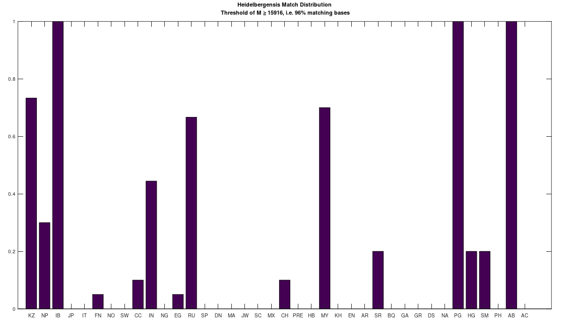

However, this is not true for lower threshold values below 96%, as the global alignment algorithm quickly produces a much more dense distribution for all populations. For example, below are the same two distributions produced using a minimum 80% match to Heidelbergensis. As you can plainly see, the global alignment (right) is much more dense, with nearly 100% of all populations at least an 80% match to Heidelbergensis. The plain takeaway here is that using the default NIH alignment is much more meaningful, because it filters the results, forcing acknowledgment of insertions and deletions, which again, can cause drastic changes to morphology and behavior.


Also, the nearest neighbor of the Heidelbergensis genome is unchanged, whether you use the default NIH alignment, or search for the globally best alignment, suggesting again, it’s more trouble than it’s worth to search for a globally best alignment, unless you’re deliberately searching for insertions and deletions within a pair of genomes. Specifically, it takes about an hour to find the nearest neighbor of every genome using the globally best alignment, whereas it takes about 25 seconds using the single default NIH alignment. Finally, I’ll note that using the default NIH alignment allows you to reliably predict ethnicity using mtDNA alone (i.e., only the maternal line). See [1] generally. This is actually astonishing, and though I haven’t tested the question, given the distribution above on the right, I would wager you’re not going to get good results using the best global alignment, since it causes all genomes to be roughly the same, precisely because it ignores insertions and deletions.
Here’s the dataset and the code:
https://www.dropbox.com/s/ht5g2rqg090himo/mtDNA.zip?dl=0
https://www.dropbox.com/s/ojmo0kw8a26g3n5/find_sequence_in_genome.m?dl=0
https://www.dropbox.com/s/p22as65hh9brpcv/Find_Seq_CMNDLINE.m?dl=0
https://www.dropbox.com/s/f7c2j2dxseq7up7/Updated_Heidelbergensis_CMNDLINE.m?dl=0
 , where
  is some set of indexes, where another genome
  is included in the cluster if
  , you find that the average total number of matching bases between the full genome
  , and all such genomes
  bases, incrementing by
  bases each iteration, and terminating at the full genome size of
  bases (i.e.,
  genomes in the dataset over each iteration. The random indexes are strictly superior, in that the average match count for every
  of the
  bases. As a consequence, if you concentrate the selected bases in a contiguous sequence, you’re creating overlap, since once you fix
  bases will likely be partially determined. Therefore, you maximize imputation by spreading the selected bases over the entire genome. Could be there an optimum distribution that isn’t random, yet not sequential? Perhaps, but the point is, random is not only good enough, but better than sequential, and therefore, the model presented in [1] makes perfect sense.
 ,
,  , with a random starting index, and then also fixed
  . The random starting index for
  , and counted how many genomes contained the sequence
  . If random bases generate stronger imputation, then fewer genomes should contain the sequence
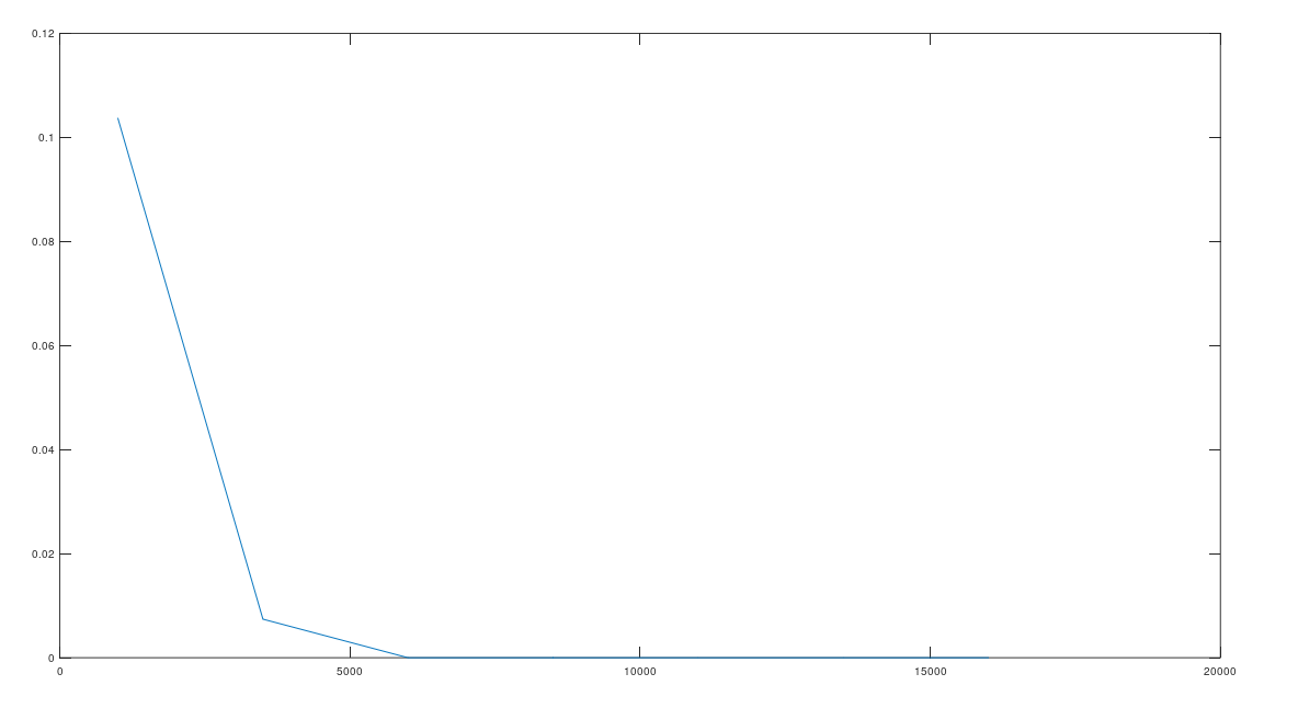

 . In the case of a single observation of a given system, Information is assumed to be given by the maximum entropy of the system given its states, and so a system with
  possible states has an Information of
  . The Uncertainty is instead given by the entropy of the distribution of states, which could of course be less than the maximum entropy given by
  . If it turns out that
  , then
  . All of this makes intuitive sense, since, e.g., a low entropy distribution carries very low Uncertainty, since it must have at least one high probability event, making the system at least somewhat predictable.