I’ve put together a very simple model of genetic inheritance that mimics sexual reproduction. The basic idea is that parents meet randomly, and if they satisfy each other’s mating criteria, they have children that then participate in the same population. Individuals die at a given age, and the age of mortality is a function of genetic fitness, and overall it’s already pretty good, though I have planned improvements.

However, that’s not what’s important, though I will follow up tonight with more code, and instead, I stumbled upon what looks like a theorem of maximizing fitness through sexual reproduction. Specifically, if individuals mate by setting a minimum total fitness that is approximately the same as theirs (i.e., my mate is roughly as fit, overall, as I am), and that mate is at the same time maximally genetically distinct from the individual in question, then you maximize the fitness of the population. So to be crude, if I’m short, you’re tall, but neither of us are notably short or tall. As a consequence, we have roughly the same total fitness, but maximally different individual traits.

Just imagine for example two roughly unfit people, that are nonetheless maximally distinct from one another, in that if an aspect of one individual is minimally fit, the other is maximally fit, though neither are fit in total. Their children could inherit the best of their respective genomes, provided they have a sufficiently large number of children. As a consequence, there is at least a chance they have a child that is categorically more fit than either of them. Of course most of the outcomes will not be the ideal case where the child inherits the best of both parent’s genes, but compare this to two identically unfit people (i.e., incest between twins). In that case, the chance the child will be superior to the parents is much lower, and there is also a chance the child will be inferior. As a consequence, the case where the parents are maximally different, creates at least the possibility of superior offspring.

This will be true of all levels of fitness in a population, and as a consequence, a population that seeks out diverse mates, should be categorically superior to a population that seeks out identical mates, provided the environment kills off the weakest of all populations. Moreover, without the possibility of upside, you leave open the possibility that you fail to beat entropy, and as a result, attempting to maintain the status quo could lead to annihilation. That is, there’s definitely error in genetic reproduction, and if the upside of evolution doesn’t outstrip the downside of error, it’s at least plausible that the species just dies due to failure to evolve.

You can also think about this in terms of financial markets, specifically, by maximizing diversity between mating partners, but being reasonable with respect to total fitness, you increase the spread of outcomes, creating both upside and downside. If the environment kills the downside (which it definitely does in Nature), you leave the upside. In contrast, a homogenous strategy would be at best where it started, creating no upside, and leaving the downside for dead. If there’s error during reproduction, which there definitely is, then that alone could wipe out a homogenous strategy. The net point being, risk is necessary for survival, because without it, you don’t produce the upside that is necessary for survival to beat error, which is analogous to beating inflation. Continuing with this analogy, there’s a window of risk, within which, you get free genetic money, because Nature is so skewed against weakness, risk creates net returns within that window.

We can make this more precise by considering two genomes A and B, and assuming that alleles are selected from either A or B with equal probability, and corresponding to traits in the child of A and B. If we list the genes in order, along the genomes, we can assign each a rank of fitness at each index. Ideally, at a given index, we select the gene that has the higher of the two rankings (e.g., if A(i) > B(i), the child has the trait associated with A(i)). Because this process is assumed to be random, the probability of success equals the probability of failure, in that the better of the two genes is just as likely to be selected as the lesser of the two genes. As a consequence, there will be an exact symmetry in the distribution of outcomes, in that every pattern of successes and failures has a corresponding compliment. This is basically the binomial distribution, except we don’t care about the actual probabilities, just the symmetry, because the point again above is that lesser outcomes are subject to culling by the environment. Therefore, Nature should produce a resultant distribution that is skewed to the upside.

Note that this is in addition to the accepted view regarding the benefits of diversity, which is that diseases can be carried by mutated bases or genes, and because genetic diseases are often common to individual populations, mating outside your population reduces the risk of passing on the genetic diseases to children. It is instead, at least for humanity, a reproductive strategy that made sense a long time ago, when we were still subject to the violence of Nature. Today, diversity is instead more sensibly justified by the fact that it reduces the risk of inheriting genetic diseases. Note that wars are temporary in the context of human history, which is the result of hundreds of thousands of years of selection, and as such, mating strategies predicated upon the culling effect of Nature or other violence don’t really make sense anymore.

Here’s the code that as I noted is not done yet, but gets you there on intuition:

https://www.dropbox.com/s/1jp616fvcs2bxvx/Sexual%20Reproduction%20CMDNLINE.m?dl=0

https://www.dropbox.com/s/li0ilkvs8a3lmg0/update_mating.m?dl=0

https://www.dropbox.com/s/shzpgw85zv2uzla/update_mortality.m?dl=0

I read an article about recent upheaval in Melanesia, specifically, that the people of Bougainville are ethnically closer to the people of the Solomon Islands, than they are to the people of Papua New Guinea. The people of Papua New Guinea are a 99% match to the Iberian Roma, and both are in turn very closely related to Heidelbergensis. See Section 6.1 of A New Model of Computational Genomics [1]. This sounds superficially implausible, but the Roma are from India, and so it’s perfectly sensible that many of them settled in Papua New Guinea.

I thought I would look into the genetics of the people of the Solomon Islands, and I found this genome in the NIH Database. It turns out the maternal line of this Solomon Island individual is completely different from that of the people of Papua New Guinea, and in fact, the individual doesn’t match to a single genome from Papua New Guinea. These are completely different people, despite superficial similarities.

Above is a chart that shows the distribution of 99% matches by population for the Solomon Islands genome. The x-axis shows the population acronym (you can find the full population name at the end of [1]), and the y-axis shows the percentage of the population in question that is a 99% match to the Solomon Islands genome. You can plainly see that this individual is closely related to many Mexicans and Hungarians. This is a truly complex world, and our notions of race are just garbage. You can find the software to build this graph in [1], and there are links to the full mtDNA dataset as well.

I downloaded this Saqqaq genome from the NIH and built clusters of genomes that are a 99% match to the Saqqaq genome, and as you can plainly see, many modern Europeans are a 99% match. The Saqqaq lived in Greenland about 4,500 years ago. I’ve seen some reports lately questioning the origins of native peoples in the Western Hemisphere, and in my work, it’s clear, that many of them are of the same maternal line as Europeans. The exception is the Mayans, who are instead related to the Iberian Roma. Here’s the distribution of 99% matches to the single Saqqaq genome. The y-axis gives the percentage of genomes in the population that are a 99% match.

I ran an algorithm on the full dataset that finds the best global alignment when comparing two genomes. I applied this to a complete Heidelbergensis mtDNA genome, comparing it to all other mtDNA genomes in the dataset below (405 complete genomes), and it turns out, you get exactly the same population using the default NIH alignment. See Section 1.3 of Vectorized Computational Genomics [1], for a discussion of the default NIH alignment. Note that the acronyms for the population names in the graphs below can also be found at the end of that paper. Specifically, on the left below is the distribution of genomes that are at least a 96% match with Heidelbergensis using the default NIH alignment, and on the right is the distribution of genomes that are at least a 96% match with Heidelbergensis using the global alignment that maximizes the number of matching bases. The latter is achieved by shifting the genome one index at a time, and counting matching bases. Because mtDNA is circular, the bases that go past the end of the genome are pushed back to the beginning in a loop. The obvious conclusion is that these populations really are anomalously closely related to Heidelbergensis.

However, this is not true for lower threshold values below 96%, as the global alignment algorithm quickly produces a much more dense distribution for all populations. For example, below are the same two distributions produced using a minimum 80% match to Heidelbergensis. As you can plainly see, the global alignment (right) is much more dense, with nearly 100% of all populations at least an 80% match to Heidelbergensis. The plain takeaway here is that using the default NIH alignment is much more meaningful, because it filters the results, forcing acknowledgment of insertions and deletions, which again, can cause drastic changes to morphology and behavior.

Also, the nearest neighbor of the Heidelbergensis genome is unchanged, whether you use the default NIH alignment, or search for the globally best alignment, suggesting again, it’s more trouble than it’s worth to search for a globally best alignment, unless you’re deliberately searching for insertions and deletions within a pair of genomes. Specifically, it takes about an hour to find the nearest neighbor of every genome using the globally best alignment, whereas it takes about 25 seconds using the single default NIH alignment. Finally, I’ll note that using the default NIH alignment allows you to reliably predict ethnicity using mtDNA alone (i.e., only the maternal line). See [1] generally. This is actually astonishing, and though I haven’t tested the question, given the distribution above on the right, I would wager you’re not going to get good results using the best global alignment, since it causes all genomes to be roughly the same, precisely because it ignores insertions and deletions.

Here’s the dataset and the code:

https://www.dropbox.com/s/ht5g2rqg090himo/mtDNA.zip?dl=0

https://www.dropbox.com/s/ojmo0kw8a26g3n5/find_sequence_in_genome.m?dl=0

https://www.dropbox.com/s/p22as65hh9brpcv/Find_Seq_CMNDLINE.m?dl=0

https://www.dropbox.com/s/f7c2j2dxseq7up7/Updated_Heidelbergensis_CMNDLINE.m?dl=0

I’m still analyzing the mtDNA Dataset I’ve been working on, and I discovered that about 3.7% of the genomes exhibit properties consistent with significant mutations from an ancestor. This is also true of the genomes that have a roughly 70% match to Denisovan mtDNA, which includes many Ashkenazi Jews. Because mtDNA is inherited as a single entire genome, with only few if any mutations, it must be the case that these populations were the result of significant selection, there’s simply no other credible argument to the contrary. Because mtDNA is fundamental to the production of ATP (i.e., energy), it’s reasonable to conclude that these populations are extremely fit, for the simple reason, that again, they must have engaged in selection over significant periods of time. Keep in mind, many living people are today a 99% match to a 4,000 year old Ancient Egyptian genome, suggesting that in the absence of mutation and selection, mtDNA really doesn’t change much. If you’re selecting mtDNA mutations, it’s fair to conclude that you’re selecting for overall health and energy, which is possibly connected to brain power as well. There are thankfully some Finnish athletes in the NIH Database, and many Finns are also closely related to Denisovans, though again, the match count is roughly 70%, implying again significant mutation and selection. Note however the populations that exhibit significant mutations are geographically widespread, and I noted the Denisovans, only because it’s such an obvious case, as you have a literally archaic bloodline, that plainly underwent significant mutation and selection. I will follow up with something more formal shortly.

Yesterday I presented even more evidence that you get stronger imputation using random bases in a genome, as opposed to sequential bases in a genome. I already presented some evidence for this claim in my paper A New Model of Computational Genomics (see Section 7) [1]. Specifically, I showed in [1] that when calculating the nearest neighbor of a partial genome, you are more likely to map to the true nearest neighbor if you use random bases, as opposed to sequential bases. This suggests that imputation is stronger when using a random set of bases, as opposed to a sequential set of bases. The purpose of Section 7 was to show that using random bases is at least workable, because the model presented is predicated upon the assumption that you don’t need to look for genes or haplogroups to achieve imputation, so I didn’t really care whether or not random bases are strictly superior, though it seems that they are.

Specifically, if you build clusters using a partial genome , where is some set of indexes, where another genome is included in the cluster if , you find that the average total number of matching bases between the full genome , and all such genomes , is greater when is a random set of indexes, versus a sequential set of indexes. 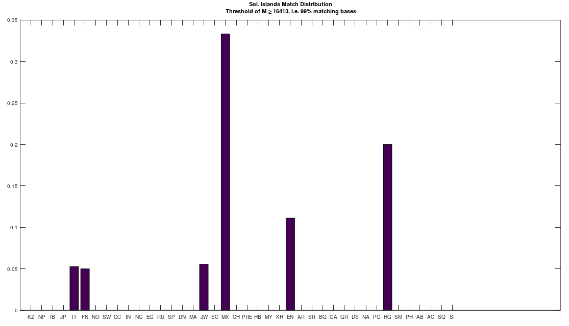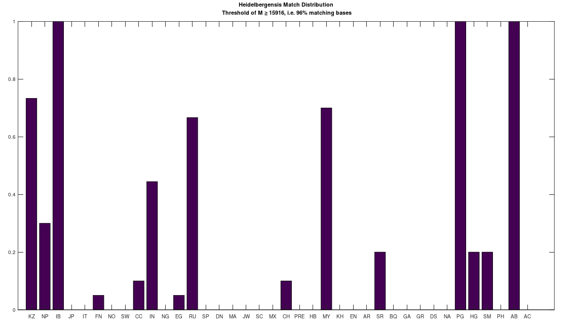Specifically, I tested this for random and sequential indexes, beginning with partial genomes of bases, incrementing by bases each iteration, and terminating at the full genome size of bases (i.e., starts out with indexes), building clusters for each of the genomes in the dataset over each iteration. The random indexes are strictly superior, in that the average match count for every of the genomes, and the genomes in their respective clusters, is higher when using random indexes, versus sequential indexes. Note that the sequential indexes have a random starting point, and as such, this is not the result of an idiosyncratic portion of the genome.

This might seem surprising, since so much of genetics is predicated upon genes and haplogroups, but it makes perfect sense, since, e.g., proteins are constructed using sequences of bases. As a consequence, if you concentrate the selected bases in a contiguous sequence, you’re creating overlap, since once you fix base, the following bases will likely be partially determined. Therefore, you maximize imputation by spreading the selected bases over the entire genome. Could be there an optimum distribution that isn’t random, yet not sequential? Perhaps, but the point is, random is not only good enough, but better than sequential, and therefore, the model presented in [1] makes perfect sense.

Here’s the dataset and the code:

https://www.dropbox.com/s/ht5g2rqg090himo/mtDNA.zip?dl=0

https://www.dropbox.com/s/9itnwc1ey92bg4o/Seq_versu_Random_Clusters_CMDNLINE.m?dl=0

In my most recent paper, A New Model of Computational Genomics [1], I showed that a genome is more likely to map to its true nearest neighbor, if you consider a random subset of bases, versus a sequential set of bases. Specifically, let be a vector of integers, viewed as the indexes of some genome. Let be a genome, and let denote the bases of , as indexed by , within . That is, is the subset of the full genome , limited to the consideration of the bases identified in . We can then run Nearest Neighbor on , which will return some genome . If is the full set of genome indexes, then will be the true nearest neighbor of .

The results in Section 7 of [1] show that as you increase the size of , you end up mapping to the true nearest neighbor more often, suggesting that imputation becomes stronger as you increase the number of known bases (i.e., the size of ). This is not surprising, and my real purpose was to prove that statistical imputation (i.e., using random indexes in ) was at least acceptable, compared to sequential imputation (i.e., using sequential indexes in ), which is closer to searching for known genes, and imputing remaining bases. It turns out random bases are actually strictly superior, which you can see below.

It turns out imputation seems to be strictly superior when using random bases, as opposed to sequential bases. Specifically, I did basically the same thing again, except this time I fixed a sequential set of bases of length , , with a random starting index, and then also fixed random bases . The random starting index for is to ensure I’m not repeatedly sampling an idiosyncratic portion of the genome. 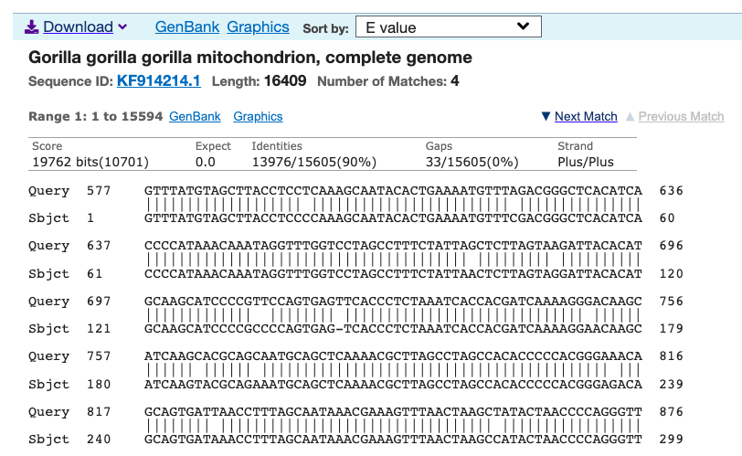I then counted how many genomes contained the sequence , and counted how many genomes contained the sequence . If random bases generate stronger imputation, then fewer genomes should contain the sequence . That is, if you get better imputation using random bases, then the resultant sequence should be less common, returning a smaller set of genomes that contain the sequence in question. This appears to be the case empirically, as I did this for every genome in the dataset below, which contains complete mtDNA genomes from the National Institute of Health.

Attached is code that lets you test this for yourself. Below is a plot that shows the percentage of times sequential imputation is superior to random imputation (i.e., the number of success divided by 405), as a function of the size of , which starts out at bases, increases by bases per iteration, and peaks at the full genome size of bases. You’ll note it quickly goes to zero.

This suggests that imputation is local, and that by increasing the distances between the sampled bases, you therefore increase the strength of the overall imputation, since you minimize the intersection of any information generated by nearby bases. The real test is actually counting how many bases are in common outside a given , and testing whether random or sequential is superior, and I’ll do that tomorrow.

https://www.dropbox.com/s/9itnwc1ey92bg4o/Seq_versu_Random_Clusters_CMDNLINE.m?dl=0

https://www.dropbox.com/s/ht5g2rqg090himo/mtDNA.zip?dl=0

My paper Information, Knowledge, and Uncertainty [1] implies the superficially awkward conclusion that a perfectly consistent set of observations, carries no Knowledge at all. This follows from the fundamental equation in [1], which assumes that Knowledge is the balance of Information less Uncertainty. Symbolically,

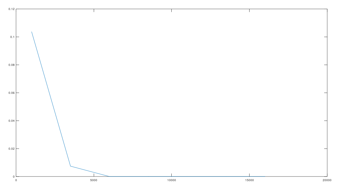
which in turn implies that . In the case of a single observation of a given system, Information is assumed to be given by the maximum entropy of the system given its states, and so a system with possible states has an Information of . The Uncertainty is instead given by the entropy of the distribution of states, which could of course be less than the maximum entropy given by . If it turns out that , then . All of this makes intuitive sense, since, e.g., a low entropy distribution carries very low Uncertainty, since it must have at least one high probability event, making the system at least somewhat predictable.

The strange case is a truly certain event, which would cause the entropy of the distribution to be zero. This in turn sets all measures to zero, implying zero Information, Knowledge, and Uncertainty. However, this makes sense if you accept Shannon’s measure of entropy, since a source with a single certain event requires zero bits to encode. Similarly, a source with a single certain event carries no Uncertainty, for exactly that reason. You could use this to argue that there’s a special case of the equation above that doesn’t really make any sense, but this is actually wrong. Specifically, you still have to have a system in the first instance, it’s just in a constant state. Such systems are physically real, albeit temporarily, e.g., a broken clock. Similarly, a source that generates only one signal still has to exist in the first instance. And as such, you have no Uncertainty with respect to something that is actually extant. In contrast, when you have no Uncertainty with respect to nothing, that’s not really notable in any meaningful or practical way. The conclusion being, that zero Knowledge coupled with zero Uncertainty, with respect to a real system, is physically meaningful, because it means that you know its state with absolute certainty. You have the maximum possible Knowledge, it just happens to be, that quantity is zero in the case of a static system.

At the risk of being overly philosophical, if we consider the set of all mathematical theorems, which must be infinite in number for the simple reason that trivial deductions are themselves theorems, then we find a fixed set, which is immutable. As a consequence, perfect Knowledge of that set would have a measure of zero bits. To make this more intuitive, consider the set of all mathematical statements, and assign each a truth value of either true or false. If you do not know the truth value of each statement, then you are considering what is from your perspective a dynamic system, which could change as information becomes available (e.g., you prove a statement false). If instead you do know the truth value of each statement, then it is a fixed system with zero Uncertainty, and therefore zero Knowledge.

I think I’m finally done with my work on mtDNA, which I’ve summarized in my paper, A New Model of Computational Genomics, though I spent some time today thinking about how it is that significant mutations occur. Specifically, if you run a BLAST Search on a human mtDNA genome, and you compare that to a gorilla, you’ll see that there’s a 577 base sequence that humans have, that gorilla’s do not, suggesting that humans are the result of a 577 base insertion into the mtDNA of a gorilla. You get a similar result with chimps and other similar species. Here’s a screen shot of a BLAST Search I ran comparing this human mtDNA genome to a gorilla’s, and you can see the Query genome (i.e., the human genome) begins at index 577, and the Subject genome (i.e. the gorilla genome) begins at index 1, suggesting that the human genome contains 577 bases that are simply absent from the gorilla genome.

This isn’t necessarily the case, but the result is consistent with the assumption that a significant insertion into a gorilla’s mtDNA, produced human mtDNA. This is obviously also consistent with evolution, but the question is, how could such a massive error occur in a healthy species? I think the answer is that it’s not a normal insertion, and instead, an already assembled, yet free-floating segment of DNA ends up attached to the end of a strand that is being assembled. That is, there’s some detritus floating around, that is an already formed strand of DNA, that ends up attached to one of the ends of another strand that is in the process of being assembled. This shouldn’t occur often either, but if it did, it wouldn’t imply that the genetic machinery is broken, which would almost certainly be the case given an insertion that is 577 bases long. That is, if it just happened to be the case that some left over strand ends up attached to another strand in the midst of being assembled, then that’s just a low probability event that is not indicative of anything wrong. In contrast, if there’s an inadvertent 577 base insertion, then the genetic machinery is broken, and will almost certainly produce lethal diseases in short order.

That said, this exogenous insertion must also not be deleterious, in order for it to persist. This is of course perfectly consistent with evolution, and at the same time, consistent with a modern understanding of genetic replication, where small errors often produce disastrous and even lethal diseases. The net result would be, a healthy species just happened to experience an unlikely event that caused a piece of stray DNA to become attached to another piece during replication, and this exogenous insertion turned out to be either benign or beneficial. This would allow for significant mutations, possibly allowing for one species to mutate into another.

I’ve been writing about alignment quite a bit lately, since my method of genomics makes use of a very simple alignment that follows the default NIH alignment, which you can see looking at the opening bases of basically any genome. This makes things really simple, and allows you to quickly compare entire genomes. However, I noted that in the case of my method of ancestry analysis, you actually should at least consider the possibility of local alignments, even though it doesn’t seem to matter very much.

I’m now convinced you should not consider local alignments unless you’re looking for genes, insertions, or deletions, because as I suspected, it turns out that insertions and deletions appear to define maternal lines. Moreover, insertions and deletions are associated with drastic changes in behavior and morphology, e.g., Down Syndrome and Williams Syndrome, unlike single-base mutations, which can cause diseases, but it’s obvious that plenty of people differ by many bases over even ideal alignments, so they’re plainly not as important as indels.

Specifically, I wrote an algorithm that iterates over every possible global alignment between two genomes, and for the Iberian Roma population (a nearly perfectly homogenous population), the alignment that maximizes the number of matching bases, when comparing two genomes from that population, is the default NIH alignment. The Iberian Roma are very closely related to the people of Papua New Guinea, and the same is true of them. However, for the Kazakh and Italian populations, this is not the case, with many genomes requiring some changes to alignment, implying insertions and deletions. These insertions and deletions therefore in turn plainly define different maternal lines within a given population, and among populations. As a consequence, again, I think the right method is to fix the global alignment using the default NIH alignment, and then compare entire genomes.

Attached is the dataset, and some code that runs through every possible global alignment.

https://www.dropbox.com/s/ht5g2rqg090himo/mtDNA.zip?dl=0

https://www.dropbox.com/s/4h1myonndzkgfts/Count_Matching_Bases.m?dl=0

https://www.dropbox.com/s/ojmo0kw8a26g3n5/find_sequence_in_genome.m?dl=0

https://www.dropbox.com/s/p22as65hh9brpcv/Find_Seq_CMNDLINE.m?dl=0