Ancient mtDNA in the Americas

Introduction

I’ve been analyzing ancient mtDNA from the Americas using the techniques that I’ve started to truly formalize (see this note from earlier today), and it’s yielded some fascinating and unquestionable findings. Specifically, there were at least three distinct genetic groups that settled the Americas, with wildly different roots in Europe, Asia, and Africa. However, I’ll begin with a somewhat formal review to help with the epistemology, and intuition.

The methods I’ve been using are easy to understand, but require a bit of thinking and analysis to understand why they work. Specifically, what I’ve been doing is not that different from what the NIH’s BLAST Search does, which is to align two genomes, and then count the matching bases. However, I’ve been using a fixed alignment that is almost always used by the NIH anyway, since I want to account for insertions and deletions, whereas the NIH simply adjusts the alignment to maximize matching bases, often ignoring insertions and deletions, and simply disregarding the atypical portion of the genome. You can read about why I think this is the right method in this note, but the overall point is that insertions and deletions are associated with drastic changes in appearance and behaviors, e.g., in cases of Down Syndrome and Williams Syndrome. As a consequence, I will not ignore them, and instead, I search for the genomes have the same structure.

In mathematical terms, a genome is a vector of labels over the set $\{A,C,G,T\}$ . As such, when comparing two genomes and counting matching bases, after adjusting alignment, we are engaging in a series of Bernoulli Trials. Therefore, the probability of generating $K$ matching bases over two genomes of length $N$ is given by the Binomial Distribution. One immediate observation after comparing any sizable number of genomes, is that mtDNA cannot be the product of chance. First note the sheer size of the outcome space, which is given by $4^N$ , where $N$ is in this case $16,576$ bases. This is a number that has approximately $10,000$ digits, and cannot be calculated using an ordinary computer. The expected number of matching bases is $\frac{1}{4} N = 4,144$ bases. The standard deviation is $\sqrt{N \frac{1}{4} \frac{3}{4}} = 55.74$ . Note that the expected number of matching bases, and the standard deviation have nothing to do with observation, and are instead implied by the fact that comparing $N$ bases is a repeated series of Bernoulli Trials, each with a probability of $\frac{1}{4}$ .

If you use the dataset attached, which consists of 205 compete human mtDNA genomes, you’ll find that taking the worst match between a given row and all others, and repeating this for each row, produces an average matching base count of about 4,500. This is about 6 standard deviations above the mean, implying that even the worst-case matches produce outcomes that cannot be credibly attributed to chance. In fact, the probabilities are so small they cannot be calculated in Octave using standard functions. Using the best-case matches (i.e., the Nearest Neighbor of each row), produces an average match count of about 16,000. This is about 213 standard deviations above the mean, plainly beyond the realm of chance. We can make sense of this by allowing for the possibility that DNA is Kolmogorov random (or close to it) in terms of its structure, yet rejecting the possibility that whether or not two genomes match is the result of chance, which is plainly not the case.

Moreover, in the note from earlier today, I showed that it doesn’t matter what portions of the genome you compare, provided that the portion compared is long enough. In fact, the results are almost always superior if the subset of the genome is randomly selected. That is, a random and possibly discontiguous sequence performs better than a contiguous sequence. This is initially counter-intuitive, since the standard method is to search for genes, and Haplogroups more generally. However, if you step back for a moment, consider being given only a fixed number of bases to analyze, which does occur because sequencing requires time, work, and money. If that limited number of indexes is randomly selected, and therefore randomly spaced, you will cover a wider portion of the genome, albeit incompletely. However, because the genome is plainly not the result of chance, the bases that are not selected are likely restricted in possibility by the bases that are selected, and as a consequence, randomly selecting some subset of bases performs better for at least some tasks. That said, obviously, the complete genome is the best performing option, so the point is instead one of epistemology, specifically, that because the genome is not random, selections constrain possibility, and as a consequence, it is at times better to cover a wider portion of the genome discontiguously, than a single contiguous sequence with the same total number of bases. Recall again, I’m not claiming that the initial construction of a genome isn’t Kolmogorov random, and I’m instead arguing that it is not the result of chance. As a consequence, given a set of genomes, the part determines the whole, and so partial information about a genome implies structure in the unobserved portion, which still allows for the overall structure to be Kolmogorov random (or close to it).

The above should provide a theoretical and practical intuition for the methods I’ve been making use of, which as you can tell, completely skip the step of identifying protein producing regions and instead focus entirely on what is common to two genomes, regardless of location or function. This is based upon the assumption that it doesn’t matter where you look in a genome, and instead the only thing that seems to matter (for at least some purposes) is the number of bases considered, and in this case, the number of matching bases between two genomes.

Application to Ancient Genomes

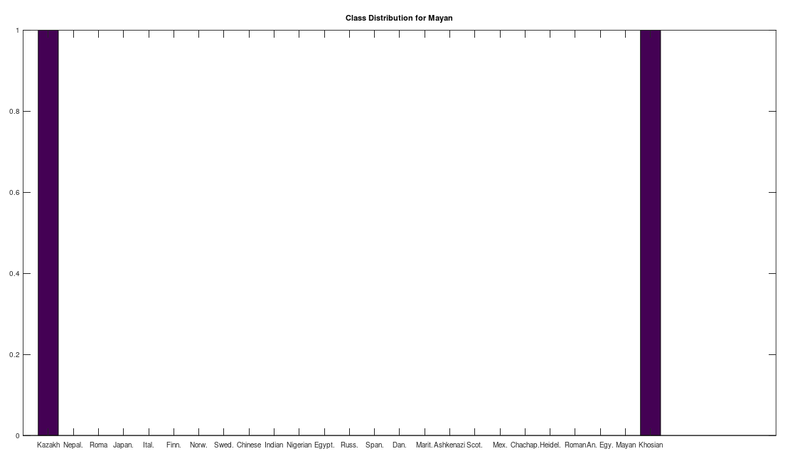
In applying these methods to Chachapoya (Peru), Mayan (Belize), and Maritime Archaic (Canada) genomes, I’ve found three distinct maternal lines. Note that all of the raw individual genomes are attached, including the assembled dataset, together with provenance files that contain links to the NIH Database for each genome. All of the genomes in the dataset are complete mtDNA genomes. The dataset includes 10 Chachapoya, 1 Mayan, and 10 Maritime Archaic genomes. I compared each row of each of the three classes to every other row in the dataset, which consists of 205 complete genomes from the following 25 groups of genomes:

[1,1] = Kazakh
[1,2] = Nepalese
[1,3] = Iberian Roma
[1,4] = Japanese
[1,5] = Italian
[1,6] = Finnish
[1,7] = Norwegian
[1,8] = Swedish
[1,9] = Chinese
[1,10] = Indian
[1,11] = Nigerian
[1,12] = Egyptian
[1,13] = Russian
[1,14] = Spanish
[1,15] = Danish
[1,16] = Maritime Archaic
[1,17] = Ashkenazi Jewish
[1,18] = Scottish
[1,19] = Mexican
[1,20] = Ancient Peruvian (Chachapoya)
[1,21] = H. Heidelbergensis
[1,22] = Ancient Roman
[1,23] = Ancien Egyptian
[1,24] = Mayan
[1,25] = Khoisan

I set the minimum match threshold to $.99 N = 16,410$ , which is at times higher than $99\%$ , since many genomes contain missing entries, which do not contribute to the threshold. Using this threshold produces the following three distributions for the Maritime Archaic, Mayan, and Chachapoya, respectively, in that order below. Keep in mind, you simply cannot argue with these results, since mtDNA does not change much from one generation to the next, and as noted above, the notion that matches on this scale are the product of chance is simply not credible, and so these groups are genetically related as set forth below. The vertical axis counts the number of times a given population matched to the population in question, and the horizontal axis gives the names of the individual populations.

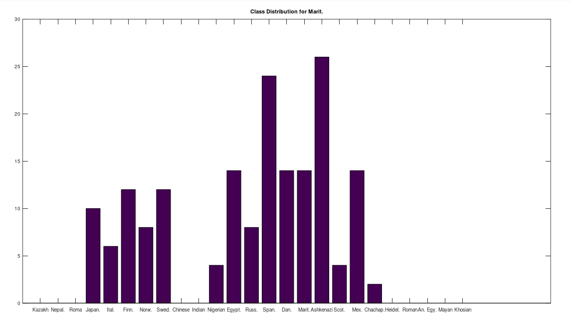
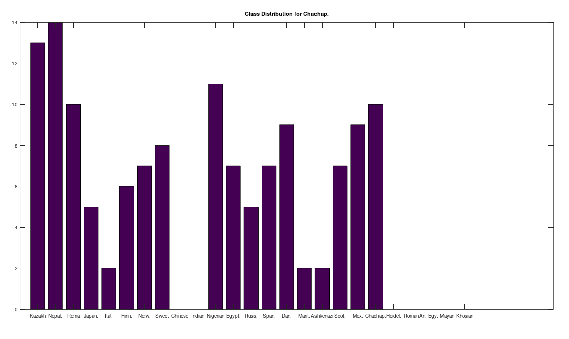
Some immediate takeaways, the Chinese and Indian populations are totally absent from these ancient American populations. This could of course be the result of the small dataset that contains only 10 genomes from each of China and India, whereas Russia is represented in both the Chachapoya and Maritime Archaic populations. If Russia were not represented, then that would be strange, given that at least some early settlers of the Americas are believed to have come over the Bering Strait. However, at a minimum, we can conclude that the Chinese and Indian maternal lines were not as well represented as the others above in the early Americas, which is not terribly surprising, since both are significantly further south than Russia.

One astonishing find, the Khoisan of Africa, believed to be one of the oldest living Homo Sapien populations, are a 99% match to the single Mayan genome. Because they are believed to be so ancient, I suppose they could end up anywhere, given the amount of time they’ve been around, but when you compare the Khoisan to the rest of the dataset, you don’t get a robust distribution, and instead get the same distribution, matching exactly once to a Kazakh genome, and the single Mayan genome, suggesting the possibility of a close genetic relationship between the Mayans and the Khoisan, and the Kazakh and the Khoisan. That is, it’s astonishing precisely because they don’t seem to be closely related to anyone else.

Another interesting note, the Iberian Roma and Nepalese people are plainly well represented in the Chachapoya population. This is very interesting, because both Iberian Roma and Nepalese are a near perfect match for Homo Heidelbergensis (approximately 97% of their mtDNA genomes are a match), an archaic human species that was thought to have gone extinct, though their maternal line plainly carries on in both populations. This suggests the possibility that Homo Heidelbergensis traveled with early Homo Sapiens to the new world, and at a minimum, that early ancestors of both the Iberian Roma and Nepalese people were present in the Americas.

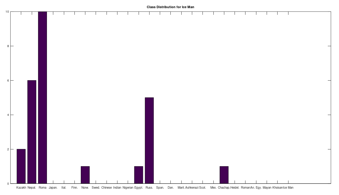
I ran the same analysis on Ötzi the Iceman, whose genome is available from the NIH, but not included in the dataset below, and it seems he is also closely related to the Iberian Roma and Nepali people, producing the following distribution: