Following up on a previous post where I introduced an algorithm to find the longest genetic sequence common to a population, I’ve now applied my most basic clustering algorithm to genetic sequences, in order to classify populations based upon genetic data, and the results are excellent, at least so far, and I’d welcome additional datasets to test this on (my software is linked to below).
The basic idea is to use A.I. clustering, to uncover populations in genetic data.
To test this idea, I created two populations, each based upon a unique genetic sequence that is 50 base pairs long, and each sequence was randomly generated, creating two totally random genetic sequences that are the “seeds” for the two populations. Each population has 100 individuals / sequences, and again, each sequence is 50 base pairs long. This ultimately creates a dataset that has 200 rows (i.e., individuals) and 50 columns (i.e., base pairs).
I then added noise to both populations, randomizing some percentage of the base pairs (e.g., swapping an A with a T). Population 1 has 2.5% of its base pairs effectively mutated using this process, and Population 2 has 5.0% of its base pairs mutated. This creates two populations that are internally heterogenous, due to mutation / noise, and of course distinct from one another (i.e., the original sequence for Populations 1 and 2 were randomly generated and are therefore distinct).
The A.I. task is to take the resultant dataset, generated by combining the two populations into a single dataset, and have the algorithm produce what are called “clusters”, which in this case means that the algorithm looks at the genetic sequence for an individual, and pulls all other sequences that it believes to be related to that individual, without “cheating” and looking at the hidden label that ultimately allows us to calculate the accuracy of the algorithm.
The algorithm in question is interesting, because it is unsupervised, meaning that there is no training step, and so the algorithm starts completely blind, with no information at all, and has to nonetheless produce clusters. This would allow for genetic data to be analyzed without any human labels at all.
This is in my opinion quite a big deal, because you wouldn’t need someone to say ex ante, that this population is e.g., from Europe, and this one is from Asia. You would instead simply let the algorithm run, and determine on its own, what individuals belong together based upon the genetic information provided, with no human guidance at all.
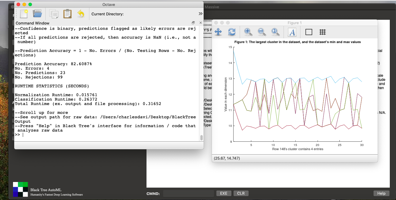
In this case, the accuracy is perfect, despite the absence of a training step, which is actually typical of my software, and there’s a set of formal proofs I presented that guarantee perfect accuracy under reasonable conditions, that are of course violated in some cases, though this (i.e., genetic datasets) doesn’t seem to be one of them. However, I’ll note that the proofs I presented (and linked to) relate to the supervised version of this algorithm, whereas I’ve never been able to formally prove why this algorithm works, though empirically it most certainly works across a wide variety of datasets. It is however very similar to the supervised version, and you can read about the supervised version here.
Finally, I’ll note that because there are only 4 base pairs, the sequences are relatively short (i.e., only 50 basepairs long), and they’re randomly generated with random noise, it’s possible to produce disastrous accuracy, using my model datasets. That is, it’s possible that the initially generated population sequences are sufficiently similar, and then noise makes this problem even worse, producing a dataset that doesn’t really have two populations. And for this reason, I welcome real world datasets, as I’m new to genetics, though not new to A.I.
 matrix, with
  sequences, and
  bases per sequence. Now assume we measure the density of each of the four bases in column i. If it turns out that the densities are given by
  for A,C,G,T, respectively, it’s reasonable to conclude that the modal base of A with a density of 0.9 is signal, and not noise, in the sense that basically all of the sequences in the dataset contain an A at that index. Moreover, the other three bases are roughly equally distributed, in context, again suggesting that the modal base of A is signal, and not noise.
 , then we could reasonably dismiss this index as noise, since the bases are uniformly distributed at that index across the entire population. In contrast, if we’re given the densities
 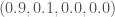 , then we should be confident that the A is signal, but we should not be as confident that the C is noise, since the other two bases both have a density of 0.
 for all four bases,
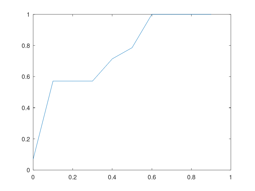
  for three bases, etc. Uncertainty is is the entropy of the distribution, and Knowledge is the balance of Information over Uncertainty,
  . Interestingly, this suggests an equivalence between Knowledge and signal, which is not surprising, as I’ve defined Knowledge as, “information that reduces uncertainty.”
 of the bases in the full sequence (i.e., the horizontal axis plots the percentage of bases fed to the Nearest Neighbor algorithm). The plot on the left uses the genome of the Influenza A virus, and the plot on the right uses the genome of the Rota virus. Both are assembled using data from the

 . Now construct a matrix
  where each column of
  such that
  , where
  maps
maps  to
to  . That is,
  , that has
  columns. That is, each of the four possible bases will have some density in each row of
  , respectively, for a given row of
  with a dimension of
  , where row
  of
of  contains the maximum entry of row
  that maps every element of
  or
or  , depending upon whether or not the entry in question is greater than some threshold in
 ![[0,1]](https://s0.wp.com/latex.php?latex=%5B0%2C1%5D&bg=ffffff&fg=444444&s=0&c=20201002) . The threshold allows us to say that if e.g., the density of A in a given row exceeds
. The threshold allows us to say that if e.g., the density of A in a given row exceeds  , then we treat it as homogenous, and uniformly A, disregarding the balance of the entries that are not A’s. It follows that the longest sequence of consecutive
  in
in  .
.