Confidence-Based Prediction

September 23, 2021May 16, 2022 / erdosfan

Summary

My core work in deep learning makes use of a notion that I call $\delta$ , which is the minimum distance over which distinction between two vectors $x,y$ is justified by the context of the dataset. As a consequence, if you know $\delta$ , then by retrieving all vectors in the dataset $y$ for which $||x - y|| \leq \delta$ , you can thereby generate a cluster associated with the vector $x$ . This has remarkable accuracy, and the runtime is $O(N)$ , where $N$ is the number of rows in the dataset, on a parallel machine. You can read a summary of the approach and the results as applied to benchmark UCI and MNIST datasets in my article, “Vectorized Deep Learning“.

Though the runtime is already fast, often fractions of a second for a dataset with a few hundred rows, you can eliminate the training step embedded in this process, by simply estimating the value of $\delta$ using a function of the standard deviation. Because you’re estimating the value of $\delta$ , the cluster returned could very well contain vectors from other classes, but this is fine, because you can then use the distribution of classes in the cluster to assign a probability to resultant predictions. For example, if you query a cluster for a vector $x$ , and get a cluster $C$ , and the mode class (i.e., the most frequent), has a density of $.5$ within $C$ , then you can reasonably say that the probability your answer is correct is $.5$ . This turns out to not work all the time, and very well sometimes, depending upon the dataset. It must work where the distribution of classes about a point is the same in the training and testing datasets, and this follows trivially from the lemmas and corollaries I present in my article, “Analyzing Dataset Consistency“. But of course, in the real world, these assumptions might not hold perfectly, which causes performance to suffer.

Another layer of analysis you can apply that allows you to measure the confidence in a given probability makes use of my work in information theory, and in particular, the equation,

$I = K + U$ ,

where $I$ is the total information that can be known about a system, $K$ is your Knowledge with the respect to the system, and $U$ is your Uncertainty with respect to the system. In this case, the equation reduces to the following:

$N \log(c) = K + N H(C)$ ,

where $N$ is the size of the prediction cluster, $c$ is the number of classes in the dataset, $K$ is again Knowledge, and $U = H(C)$ is the Shannon Entropy of the prediction cluster, as a function of the distribution of classes in the cluster.

You can then require both the probability of a prediction, and your Knowledge in that probability, to exceed a given threshold in order to accept the prediction as valid.

Knowledge is in this case given by,

$K = N \log(c) - N H(C)$ .

You can read about why these equations make sense in my paper, “Information, Knowledge, and Uncertainty“.

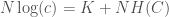
If you do this, it works quite well, and below is a plot of accuracy as a function of a threshold for both the probability and Knowledge, with Knowledge adjusted to an $[0,1]$ scale, given $5,000$ rows of the MNIST Fashion Dataset. The effect of this is to require an increasingly high probability, and increasing confidence in your measure of that probability. The dataset is then broken into $4,250$ random training and $750$ random testing rows, done $150$ times. The accuracy shown below is the average over each of the $150$ runs, as a function of the minimum threshold, which is again, applied to both the accuracy and the confidence. The reason the prediction drops to $0$ at a certain point, is because there are no rows left that satisfy the threshold. The accuracy peaks at $99.647\%$ , and again, this is without any training step, so it is in fairness, an unsupervised algorithm.